CHL5202: Biostatistics II
Course Description and Objectives
- The goal of this course is to continue development and application of skills in statistical analysis required in epidemiologic and health care research.
- Analysis where outcome is continuous and exposure and covariates are a mix of continuous and categorical variables (multiple linear regression)
- Relaxing linearity assumptions of continuous exposure variables through the use of regression splines
- Perform internal validation by means of bootstrapping or cross-validation
- Extension to binary outcomes (multiple logistic regression)
- Extension to time to event and censored outcomes (survival analysis)
- Dealing with missing data
- Introduce Bayesian methods
Course material provided by Professor Kevin Thorpe and modifications were made by myself.
Tutorial 1
Question 1
Load the data frame tut1 into R from the file
tut1.RData available on the course page. The data frame
contains the variables x and y.
Fit a simple regression with y as the response and x as the predictor. Use diagnostic plots to determine if a non-linear relationship should be modelled. If you believe a non-linear relationship is present, model it using a restricted cubic spline. The number of knots is up to you.
# Load packages and data
library(rms)
library(lattice)
library(tidyverse)

load("./CHL5202/tut1.RData")

dd <- datadist(tut1)
options(datadist="dd")
Some notes taken from here.
Comparing
ols()vslm(): one advantage forols()is that the entire variance-covariance matrix is saved
fit0 <- ols(y~x,data=tut1)
fit0
## Linear Regression Model
##
## ols(formula = y ~ x, data = tut1)
##
## Model Likelihood Discrimination
## Ratio Test Indexes
## Obs 100 LR chi2 32.07 R2 0.274
## sigma1.0827 d.f. 1 R2 adj 0.267
## d.f. 98 Pr(> chi2) 0.0000 g 0.769
##
## Residuals
##
## Min 1Q Median 3Q Max
## -2.21787 -0.73287 0.02416 0.74941 2.75329
##
##
## Coef S.E. t Pr(>|t|)
## Intercept 1.2185 0.2149 5.67 <0.0001
## x -0.3597 0.0591 -6.09 <0.0001- When applying
anovato anolsmodel, it separates out the linear and non-linear components of restricted cubic splines and polynomial terms (and product terms if they are present). - Unlike for
lm(), usinganova()withols()we have partial F-tests that describe the marginal impact of removing each covariate from the model.
anova(fit0)## Analysis of Variance Response: y
##
## Factor d.f. Partial SS MS F P
## x 1 43.43251 43.432506 37.05 <.0001
## REGRESSION 1 43.43251 43.432506 37.05 <.0001
## ERROR 98 114.88584 1.172305- Next, we check the model assumptions using diagnostic plots.
- In the Normal Q-Q Plot we are looking for normally distributed error terms, i.e. most of the points lie on the line and do not show a non-linear pattern.
# for diagnostic plots
dx0 <- data.frame(tut1, e = resid(fit0), yhat = fitted(fit0))

# Normal QQ Plot
qqnorm(dx0$e)
qqline(dx0$e)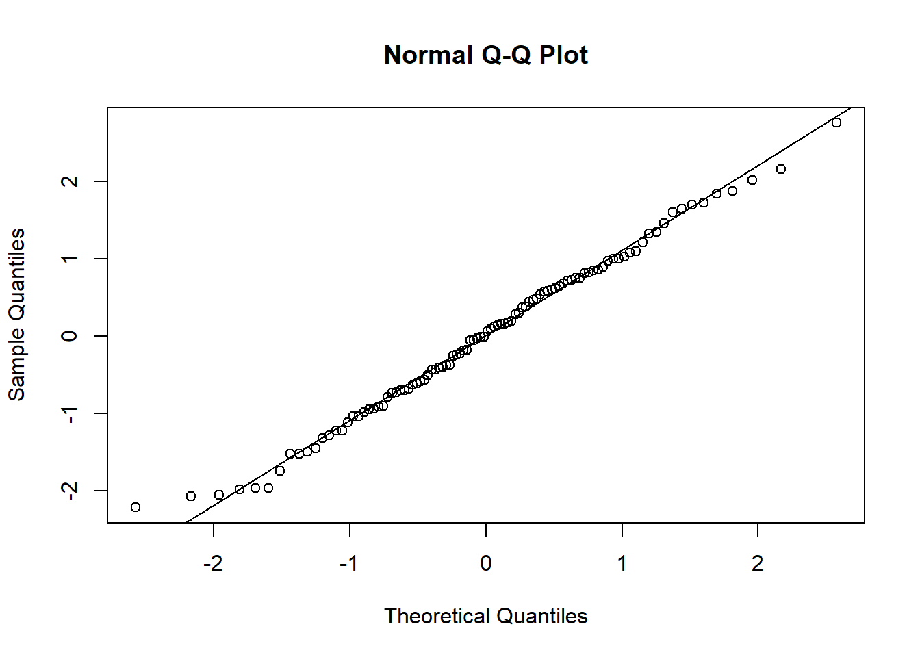
xyplot(): Common Bivariate Trellis Plots. Produces conditional scatterplots, typically between two continuous variables. Below we have residual plots.- We are looking for the residuals to not show a distinct (non-linear) pattern which would suggest that a transformation is required.
# Residual Plots
xyplot(e~x, data = dx0, type = c("p","smooth"))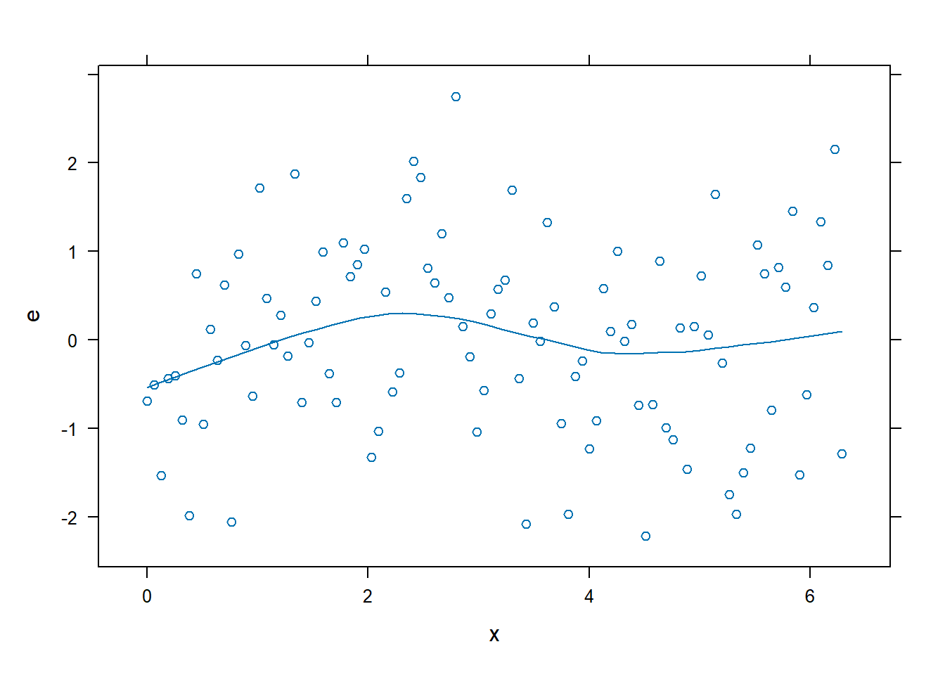
xyplot(e~yhat, data = dx0, type = c("p","smooth"))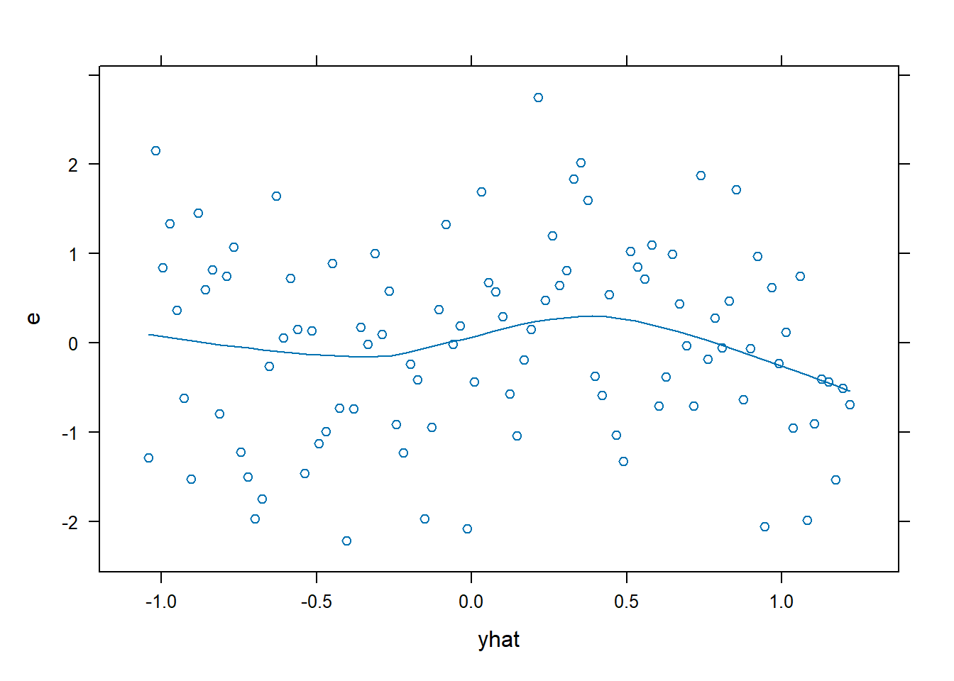
- A non-linear relationship is present, so we will model it using a restricted cubic spline. For this example, we are going to use 4 knots.
fit1 <- ols(y ~ rcs(x, 4), data = tut1)

fit1
## Linear Regression Model
##
## ols(formula = y ~ rcs(x, 4), data = tut1)
##
## Model Likelihood Discrimination
## Ratio Test Indexes
## Obs 100 LR chi2 46.60 R2 0.372
## sigma1.0173 d.f. 3 R2 adj 0.353
## d.f. 96 Pr(> chi2) 0.0000 g 0.875
##
## Residuals
##
## Min 1Q Median 3Q Max
## -2.0412 -0.7268 0.1088 0.5716 2.3664
##
##
## Coef S.E. t Pr(>|t|)
## Intercept 0.2834 0.3389 0.84 0.4050
## x 0.6559 0.2760 2.38 0.0195
## x' -3.3087 0.8566 -3.86 0.0002
## x'' 9.3222 2.4876 3.75 0.0003- It is difficult to interpret the coefficients above. The
anova()output below is more useful and shows a significant non-linear component.
anova(fit1)## Analysis of Variance Response: y
##
## Factor d.f. Partial SS MS F P
## x 3 58.97203 19.657342 19.00 <.0001
## Nonlinear 2 15.53952 7.769761 7.51 9e-04
## REGRESSION 3 58.97203 19.657342 19.00 <.0001
## ERROR 96 99.34632 1.034858# Plot predicted fit with confidence interval
ggplot(Predict(fit1))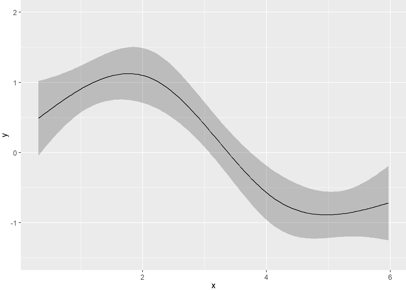
# for diagnostic plots
dx1 <- data.frame(tut1, e = resid(fit1), yhat = fitted(fit1))

# Normal QQ Plot
qqnorm(dx1$e)
qqline(dx1$e)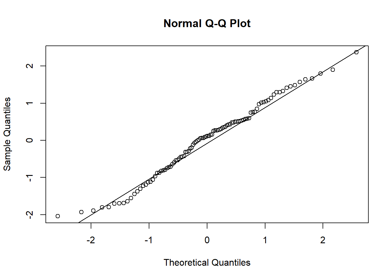
# Residual plots
xyplot(e ~ x, data = dx1, type = c("p", "smooth"))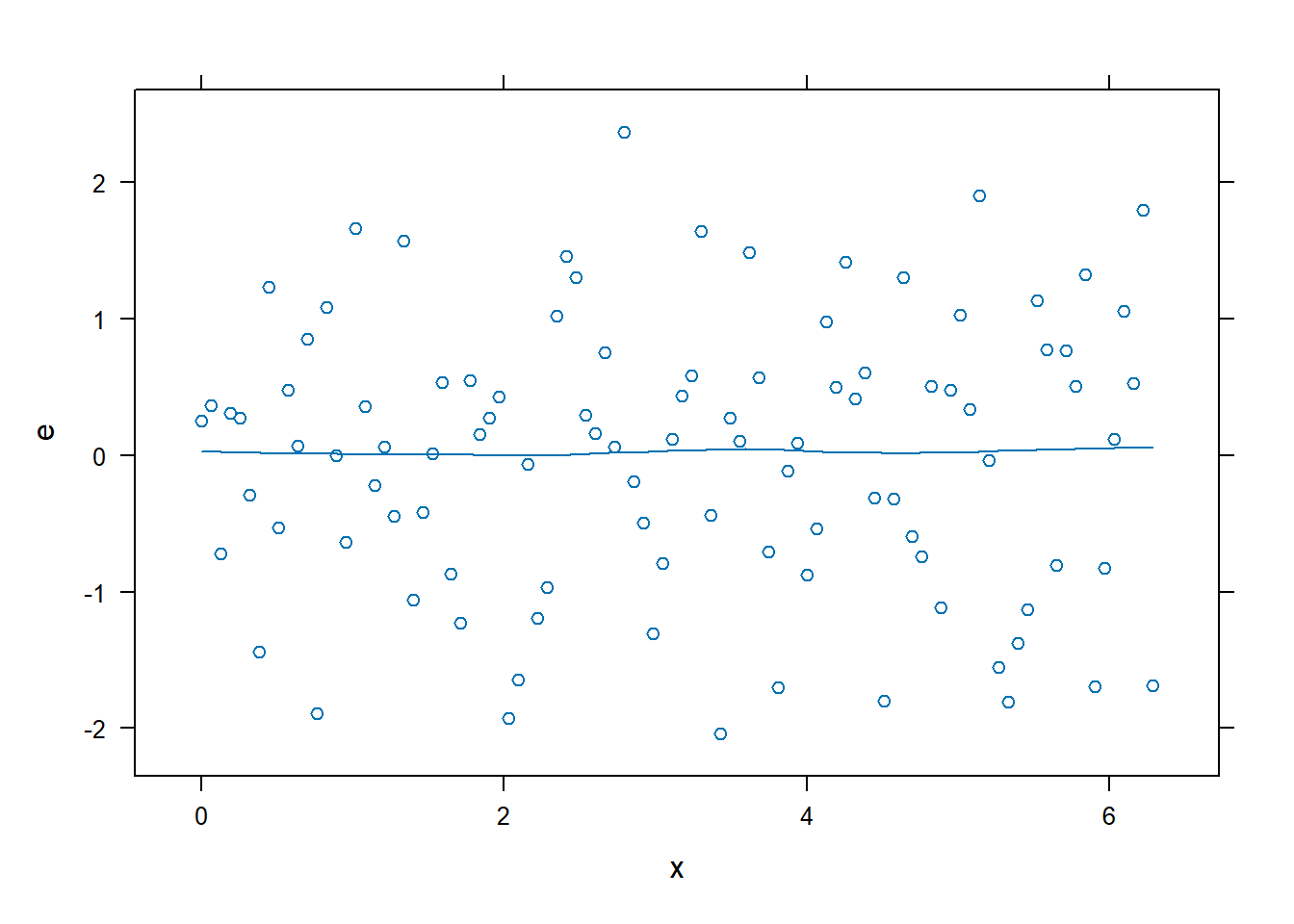
xyplot(e ~ yhat, data = dx1, type = c("p", "smooth"))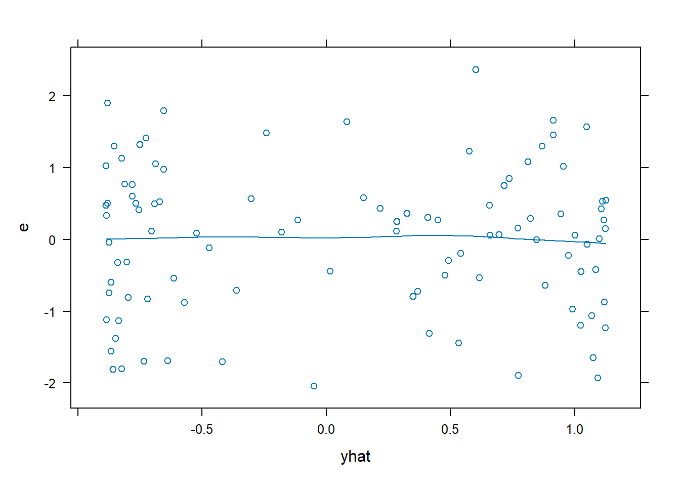
- There is no longer a non-linear pattern in the residuals.
Question 2
Load the data frame FEV from the file FEV.RData. For these data, use the variable fev as the response and the rest as the explanatory covariates.
Fit an additive linear model to fev using the other variables as the covariates. Evaluate whether any of the continuous variables should be fit as non-linear terms.
Fit an another additive model but this time model the continuous covariates with restricted cubic splines with four knots. Describe the results.
load("./CHL5202/FEV.RData")

fev.dd <- datadist(FEV)
options(datadist = "fev.dd")
# `dplyr()`: package for data wrangling - part of `tidyverse()`
library(dplyr)
# Useful for quickly viewing the data
glimpse(FEV)## Rows: 654
## Columns: 6
## $ id <int> 301, 451, 501, 642, 901, 1701, 1752, 1753, 1901, 1951, 1952, 20…
## $ age <int> 9, 8, 7, 9, 9, 8, 6, 6, 8, 9, 6, 8, 8, 8, 8, 7, 5, 6, 9, 9, 5, …
## $ fev <dbl> 1.708, 1.724, 1.720, 1.558, 1.895, 2.336, 1.919, 1.415, 1.987, …
## $ height <dbl> 57.0, 67.5, 54.5, 53.0, 57.0, 61.0, 58.0, 56.0, 58.5, 60.0, 53.…
## $ sex <fct> female, female, female, male, male, female, female, female, fem…
## $ smoke <fct> non-current smoker, non-current smoker, non-current smoker, non…summary(FEV)## id age fev height sex
## Min. : 201 Min. : 3.000 Min. :0.791 Min. :46.00 female:318
## 1st Qu.:15811 1st Qu.: 8.000 1st Qu.:1.981 1st Qu.:57.00 male :336
## Median :36071 Median :10.000 Median :2.547 Median :61.50
## Mean :37170 Mean : 9.931 Mean :2.637 Mean :61.14
## 3rd Qu.:53639 3rd Qu.:12.000 3rd Qu.:3.119 3rd Qu.:65.50
## Max. :90001 Max. :19.000 Max. :5.793 Max. :74.00
## smoke
## non-current smoker:589
## current smoker : 65
##
##
##
## # Fit initial additive model
fev.lin <- ols(fev ~ age + height + sex + smoke, data = FEV)
fev.lin## Linear Regression Model
##
## ols(formula = fev ~ age + height + sex + smoke, data = FEV)
##
## Model Likelihood Discrimination
## Ratio Test Indexes
## Obs 654 LR chi2 976.59 R2 0.775
## sigma0.4122 d.f. 4 R2 adj 0.774
## d.f. 649 Pr(> chi2) 0.0000 g 0.869
##
## Residuals
##
## Min 1Q Median 3Q Max
## -1.376562 -0.250333 0.008938 0.255879 1.920471
##
##
## Coef S.E. t Pr(>|t|)
## Intercept -4.4570 0.2228 -20.00 <0.0001
## age 0.0655 0.0095 6.90 <0.0001
## height 0.1042 0.0048 21.90 <0.0001
## sex=male 0.1571 0.0332 4.73 <0.0001
## smoke=current smoker -0.0872 0.0593 -1.47 0.1414anova(fev.lin)## Analysis of Variance Response: fev
##
## Factor d.f. Partial SS MS F P
## age 1 8.0994719 8.0994719 47.67 <.0001
## height 1 81.5049421 81.5049421 479.66 <.0001
## sex 1 3.8032782 3.8032782 22.38 <.0001
## smoke 1 0.3683978 0.3683978 2.17 0.1414
## REGRESSION 4 380.6402823 95.1600706 560.02 <.0001
## ERROR 649 110.2795540 0.1699223ageandheightare continuous variables, so we can use residual plots.sexandsmokeare categorical variables (in fact, they’re binary) so residual plots won’t be useful.
dx.fev <- data.frame(FEV, e = resid(fev.lin), yhat = fitted(fev.lin))

xyplot(e ~ age, data = dx.fev, type = c("p", "smooth"))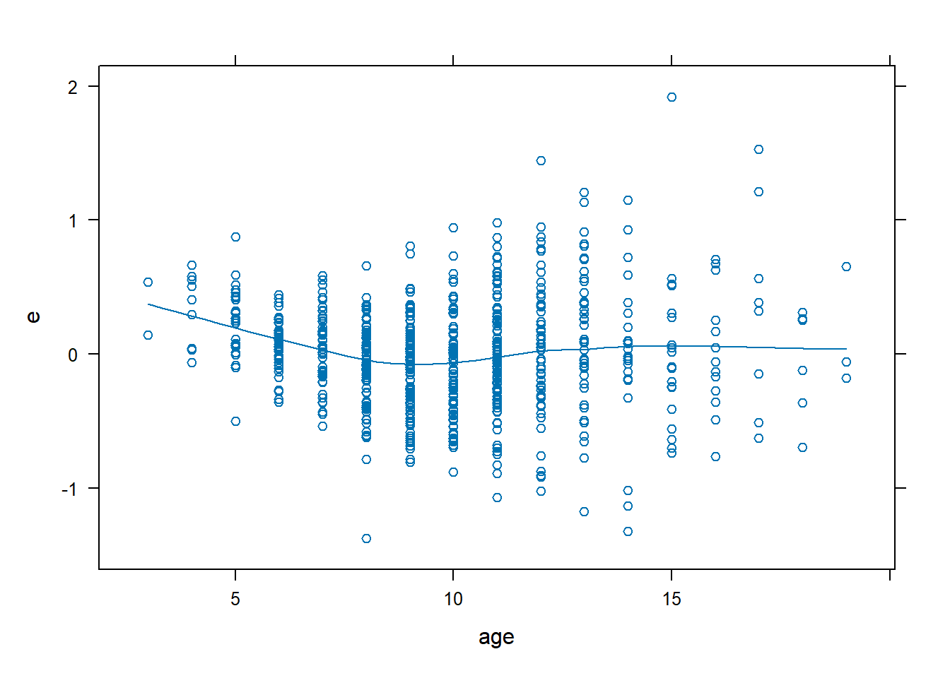
xyplot(e ~ height, data = dx.fev, type = c("p", "smooth"))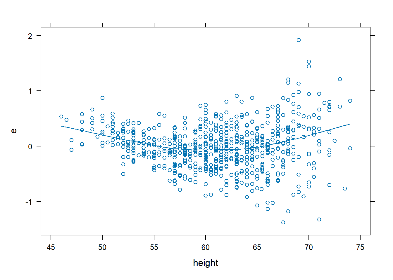
- The residual plots show that non-linearity needs to be modelled for both variables.
- Once again, we shall use restricted cubic splines with 4 knots.
fev.full <- ols(fev ~ rcs(age, 4) + rcs(height, 4) + sex + smoke, data = FEV)

fev.full
## Linear Regression Model
##
## ols(formula = fev ~ rcs(age, 4) + rcs(height, 4) + sex + smoke,
## data = FEV)
##
## Model Likelihood Discrimination
## Ratio Test Indexes
## Obs 654 LR chi2 1039.74 R2 0.796
## sigma0.3940 d.f. 8 R2 adj 0.794
## d.f. 645 Pr(> chi2) 0.0000 g 0.878
##
## Residuals
##
## Min 1Q Median 3Q Max
## -1.637487 -0.223633 0.008879 0.236143 1.776429
##
##
## Coef S.E. t Pr(>|t|)
## Intercept -2.7618 0.6718 -4.11 <0.0001
## age -0.0109 0.0343 -0.32 0.7509
## age' 0.1815 0.0733 2.48 0.0135
## age'' -0.7112 0.3094 -2.30 0.0218
## height 0.0834 0.0151 5.51 <0.0001
## height' 0.0114 0.0308 0.37 0.7114
## height'' 0.1252 0.1349 0.93 0.3540
## sex=male 0.0951 0.0335 2.83 0.0047
## smoke=current smoker -0.1485 0.0576 -2.58 0.0102anova(fev.full)## Analysis of Variance Response: fev
##
## Factor d.f. Partial SS MS F P
## age 3 10.2137671 3.4045890 21.93 <.0001
## Nonlinear 2 0.9847797 0.4923898 3.17 0.0426
## height 3 80.2711567 26.7570522 172.36 <.0001
## Nonlinear 2 3.1249430 1.5624715 10.06 <.0001
## sex 1 1.2475614 1.2475614 8.04 0.0047
## smoke 1 1.0306405 1.0306405 6.64 0.0102
## TOTAL NONLINEAR 4 10.1495441 2.5373860 16.34 <.0001
## REGRESSION 8 390.7898263 48.8487283 314.67 <.0001
## ERROR 645 100.1300100 0.1552403- The
anova()output suggests that the non-linear components for age and height are statistically significant.
dx.full <- data.frame(FEV, e = resid(fev.full), yhat = fitted(fev.full))

# Residual plots look good
xyplot(e ~ age, data = dx.full, type = c("p", "smooth"))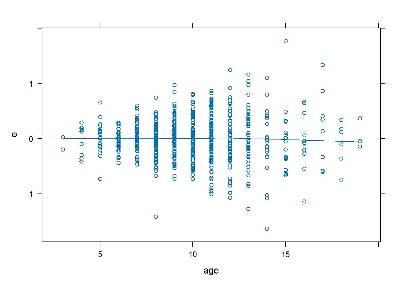
xyplot(e ~ height, data = dx.full, type = c("p", "smooth"))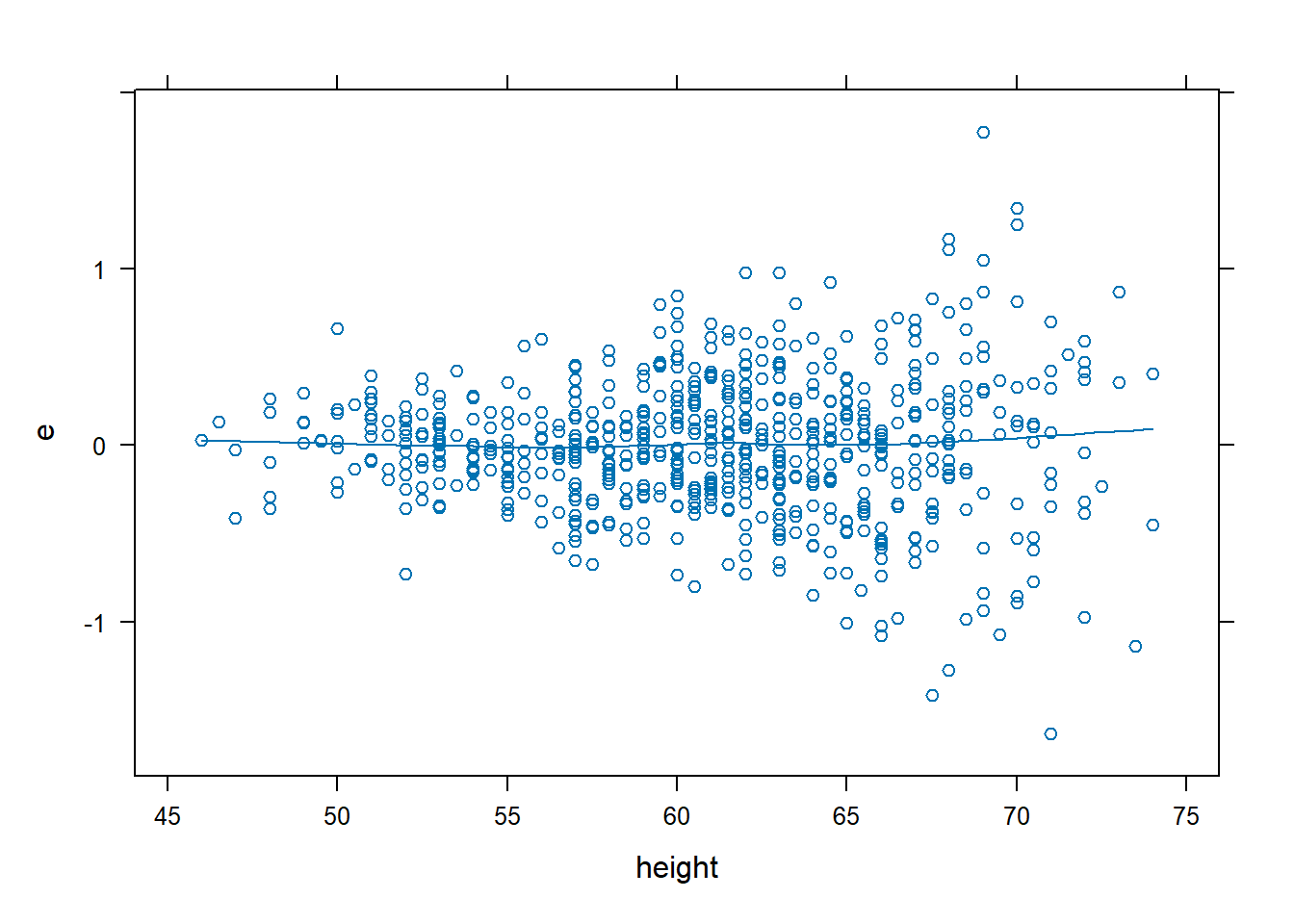
- Running
summary()is the best way to get the effects of the categorical variables. - For continuous variables, it is better to plot.
summary(fev.full)## Effects Response : fev
##
## Factor Low High Diff. Effect S.E.
## age 8 12.0 4.0 0.344100 0.059919
## height 57 65.5 8.5 0.888570 0.061187
## sex - female:male 2 1.0 NA -0.095061 0.033533
## smoke - current smoker:non-current smoker 1 2.0 NA -0.148540 0.057649
## Lower 0.95 Upper 0.95
## 0.22644 0.461760
## 0.76842 1.008700
## -0.16091 -0.029214
## -0.26174 -0.035337ggplot(Predict(fev.full, age))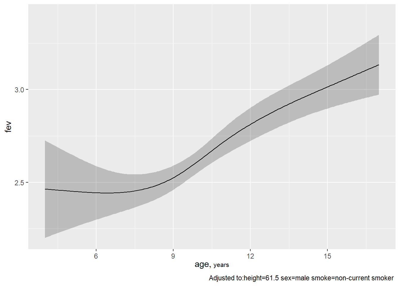
ggplot(Predict(fev.full, height))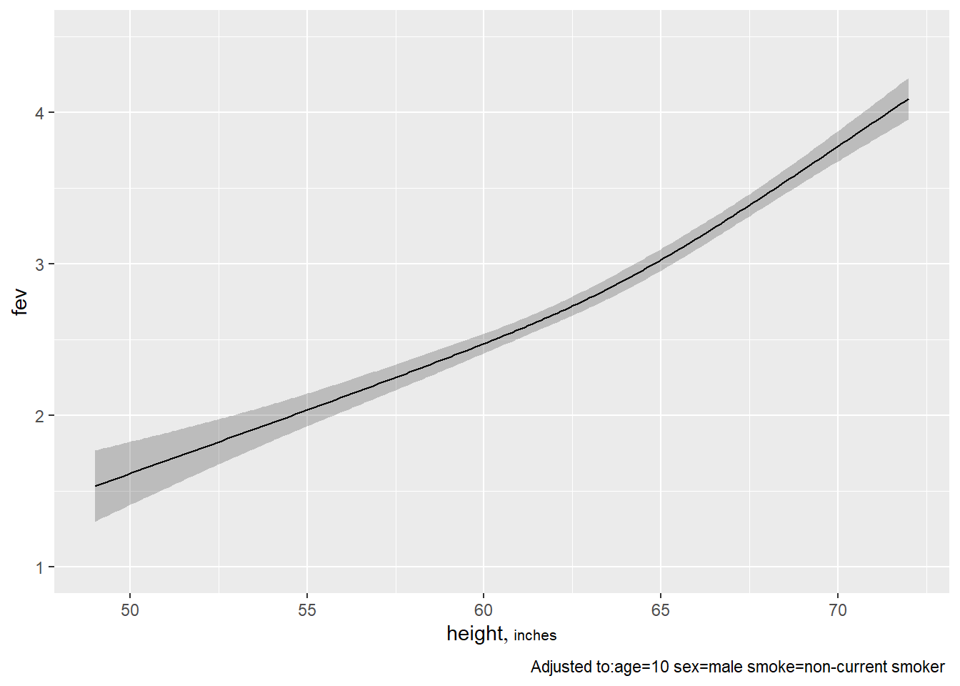
Extra
%>%: pipe operator - very useful for performing multiple data wrangling stepsggplot2(): plotting package, included inrms()andtidyverse()
# Boxplot
FEV %>%
  ggplot(mapping = aes(x = sex, y = height, fill = sex)) +
  geom_boxplot() +
  theme_bw() +
  labs(title = "Boxplot of heights by sex")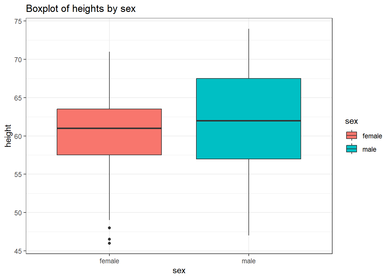
Tutorial 2
Question 1
Use the hwy2.RData file available from the course page. After
attaching the rms package and doing the usual
datadist()/options() task, fit the following model:
fit <- ols(rate~rcs(trks,4)+rcs(sigs1,4)+type+hwy,data=hwy2,x=TRUE,y=TRUE)
Run both the ordinary bootstrap validation and the .632 bootstrap validation on this model. Use the same number of iterations and seed for both validations (to compare the results). What are your conclusions?
library(rms)

load("./CHL5202/hwy2.RData")

h.dd <- datadist(hwy2)
options(datadist="h.dd")

fit <- ols(rate ~ rcs(trks,4) + rcs(sigs1,4) + type + hwy, data=hwy2, x=TRUE, y=TRUE)
# Standard bootstrap
set.seed(321) # Set seed is reproducibility. Choose any number you like.
validate(fit, B=100)##
## Divergence or singularity in 11 samples## index.orig training test optimism index.corrected n
## R-square 0.7110 0.7802 0.3163 0.4640 0.2471 89
## MSE 1.1106 0.7859 2.6277 -1.8418 2.9523 89
## g 1.8604 1.8808 1.6933 0.1876 1.6728 89
## Intercept 0.0000 0.0000 0.6535 -0.6535 0.6535 89
## Slope 1.0000 1.0000 0.8493 0.1507 0.8493 89# .632 bootstrap
set.seed(321)
validate(fit, method = ".632", B=100)##
## Divergence or singularity in 11 samples## index.orig training test optimism index.corrected n
## R-square 0.7110 0.7802 -0.3786 0.6886 0.0224 89
## MSE 1.1106 0.7859 5.0256 -2.4743 3.5849 89
## g 1.8604 1.8808 1.2664 0.3754 1.4850 89
## Intercept 0.0000 0.0000 1.2077 -0.7633 0.7633 89
## Slope 1.0000 1.0000 0.5981 0.2540 0.7460 89Conclusions:
There is a discrepancy in standard bootstrap vs .632 method – the standard bootstrap may be overfitting so we use the .632 method to double check the validation results. The .632 bootstrap applies a correction factor to reduce the bias.
Standard bootstrap may believe the model is less overfit than what it actually is, i.e. low optimism so
index.correctedis closer toindex.orig.The drop in R-square is very large from validation (went from positive to negative), indicating the original model was very overfit to the point where the relationship inverted.
Slope change seems to imply an adjusted slope estimate should be around 0.75 of what the original model guessed.
Extra
Let’s investigate the outputs from a simpler model.
# We remove the restricted cubic splines which may be the main source of overfitting
fit2 <- ols(rate ~ trks + sigs1 + type + hwy, data=hwy2, x=TRUE, y=TRUE)

set.seed(321)
validate(fit2, B=100)
##
## Divergence or singularity in 11 samples## index.orig training test optimism index.corrected n
## R-square 0.6031 0.6535 0.5132 0.1402 0.4628 89
## MSE 1.5255 1.2468 1.8708 -0.6240 2.1494 89
## g 1.6155 1.6571 1.5645 0.0926 1.5230 89
## Intercept 0.0000 0.0000 0.3534 -0.3534 0.3534 89
## Slope 1.0000 1.0000 0.9146 0.0854 0.9146 89set.seed(321)
validate(fit2, method = ".632", B=100)##
## Divergence or singularity in 11 samples## index.orig training test optimism index.corrected n
## R-square 0.6031 0.6535 0.1379 0.2940 0.3091 89
## MSE 1.5255 1.2468 2.4057 -0.5563 2.0818 89
## g 1.6155 1.6571 1.2776 0.2136 1.4019 89
## Intercept 0.0000 0.0000 0.5816 -0.3676 0.3676 89
## Slope 1.0000 1.0000 0.7459 0.1606 0.8394 89For the .632 bootstrap, the magnitude of the optimism for all 5 values is smaller than in the saturated model which showed overfitting.
Hard to say whether this model is still overfitting but it is certainly an improvement.
The R-square term in particular shows a major improvement, as the test R-square is positive rather than negative like previously shown.
Tutorial 3
Question 1
Load the data from tutdata from the file
tutdata.RData posted on the course page. Fit an additive
model where y is the outcome and the predictors are
blood.pressure, sex, age, and
cholesterol but they should use a restricted cubic spline
with four knots for cholesterol.
library(rms)
load("./CHL5202/tutdata.RData")

dd <- datadist(tutdata)
options(datadist="dd")

fit <- lrm(y ~ blood.pressure + sex + age + rcs(cholesterol,4), data = tutdata)
Question 2
Which “variables” are significant at the 5% level?
anova(fit)## Wald Statistics Response: y
##
## Factor Chi-Square d.f. P
## blood.pressure 0.33 1 0.5640
## sex 13.45 1 0.0002
## age 25.58 1 <.0001
## cholesterol 1.27 3 0.7368
## Nonlinear 0.78 2 0.6758
## TOTAL 38.63 6 <.0001- At the 5% significance level,
sexandageare statistically significant with p-values of 0.0002 and < 0.0001 respectively.
Question 3
Display the cholesterol effect.
# log odds
plot(Predict(fit,cholesterol))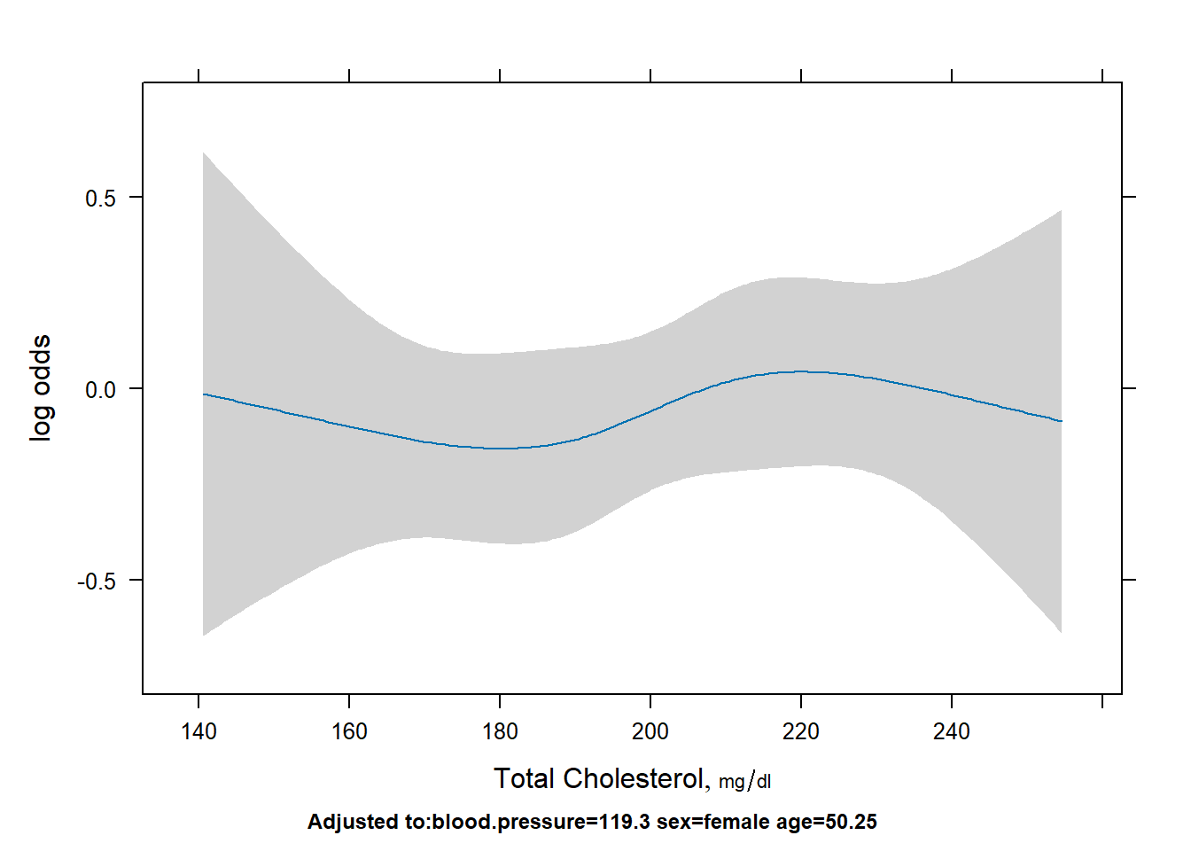
# probability
plot(Predict(fit,cholesterol,fun=plogis), ylab="Probability")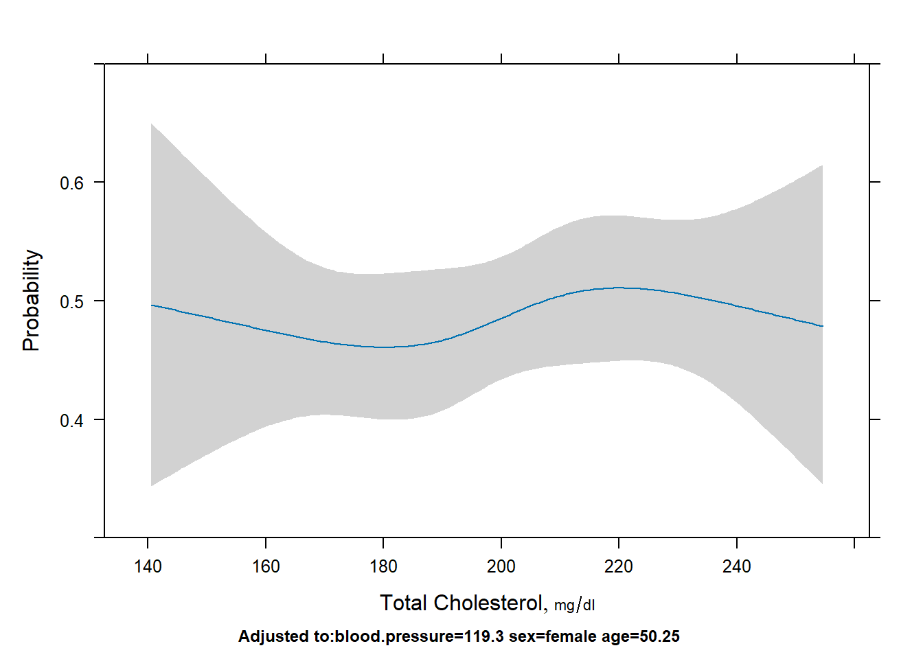
# odds
plot(Predict(fit,cholesterol,fun=exp), ylab="Odds")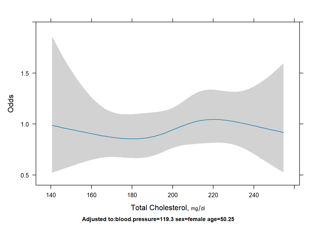
Question 4
Describe the effect of sex.
summary(fit)## Effects Response : y
##
## Factor Low High Diff. Effect S.E. Lower 0.95
## blood.pressure 109.580 130.580 20.991 -0.052121 0.090347 -0.22920
## Odds Ratio 109.580 130.580 20.991 0.949210 NA 0.79517
## age 43.531 56.677 13.146 0.438050 0.086609 0.26830
## Odds Ratio 43.531 56.677 13.146 1.549700 NA 1.30770
## cholesterol 183.730 216.530 32.796 0.194330 0.174400 -0.14748
## Odds Ratio 183.730 216.530 32.796 1.214500 NA 0.86288
## sex - male:female 1.000 2.000 NA 0.477030 0.130050 0.22213
## Odds Ratio 1.000 2.000 NA 1.611300 NA 1.24870
## Upper 0.95
## 0.12496
## 1.13310
## 0.60780
## 1.83640
## 0.53615
## 1.70940
## 0.73192
## 2.07910- The odds of the outcome
yfor males is 1.61 times the odds for females (with 95% CI [1.25,2.08]) controlled for blood pressure, age and cholesterol.
Extra
- Interpreting odds ratios for continuous variables: for every one unit increase in the continuous variable, the odds of the outcome multiply by \(\exp(\beta)\), where \(\beta\) represents the log-odds ratio.
- E.g. referring to Question 4 output: for every one year increase in age, the odds of the outcome multiply by 1.55. Alternatively, it might be more intuitive to say that the odds of the outcome increases by 55%.
Tutorial 4
Question 1
Use the data from last week (tutdata.RData) and re-fit
the model from last week which was an additive model where
y is the outcome and the predictors are
blood.pressure, sex, age, and
cholesterol except this time use a restricted cubic spline
with four knots for cholesterol. Re-run the anova also.
library(rms)
load("./CHL5202/tutdata.RData")

dd <- datadist(tutdata)
options(datadist="dd")

fit1 <- lrm(y ~ blood.pressure + sex + age + rcs(cholesterol,4), data = tutdata)
anova(fit1)
## Wald Statistics Response: y
##
## Factor Chi-Square d.f. P
## blood.pressure 0.33 1 0.5640
## sex 13.45 1 0.0002
## age 25.58 1 <.0001
## cholesterol 1.27 3 0.7368
## Nonlinear 0.78 2 0.6758
## TOTAL 38.63 6 <.0001Question 2
Fit a model as above only this time, add interactions between sex and
age as well as sex and the RCS for cholesterol and run
anova() on this model.
fit2 <- lrm(y ~ blood.pressure + sex * (age + rcs(cholesterol,4)), data = tutdata)
anova(fit2)
## Wald Statistics Response: y
##
## Factor Chi-Square d.f. P
## blood.pressure 0.26 1 0.6105
## sex (Factor+Higher Order Factors) 38.71 5 <.0001
## All Interactions 26.13 4 <.0001
## age (Factor+Higher Order Factors) 30.42 2 <.0001
## All Interactions 3.86 1 0.0495
## cholesterol (Factor+Higher Order Factors) 23.78 6 0.0006
## All Interactions 22.47 3 0.0001
## Nonlinear (Factor+Higher Order Factors) 5.33 4 0.2550
## sex * age (Factor+Higher Order Factors) 3.86 1 0.0495
## sex * cholesterol (Factor+Higher Order Factors) 22.47 3 0.0001
## Nonlinear 4.79 2 0.0911
## Nonlinear Interaction : f(A,B) vs. AB 4.79 2 0.0911
## TOTAL NONLINEAR 5.33 4 0.2550
## TOTAL INTERACTION 26.13 4 <.0001
## TOTAL NONLINEAR + INTERACTION 26.81 6 0.0002
## TOTAL 62.26 10 <.0001- All interactions with
sexare statistically significant.
Question 3
Compare the two models with a likelihood ratio test. What does it show?
lrtest(fit1,fit2)##
## Model 1: y ~ blood.pressure + sex + age + rcs(cholesterol, 4)
## Model 2: y ~ blood.pressure + sex * (age + rcs(cholesterol, 4))
##
## L.R. Chisq d.f. P
## 2.831616e+01 4.000000e+00 1.076137e-05- We are testing the null hypothesis that all of the coefficients for the interaction terms are equal to 0.
- Degrees of freedom (df): 10 df (more complicated model) minus 6 df (simpler model) equals 4 df.
- With the extremely small p-value from the likelihood ratio test, we reject the null hypothesis and conclude that at least one of the coefficients is not equal to 0.
- This p-value is equivalent to the p-value for
TOTAL INTERACTIONin theanova(fit2)output as this is what we are testing.
Question 4
Describe the sex/age and sex/cholesterol relationships with outcome.
plot(Predict(fit2,age,sex))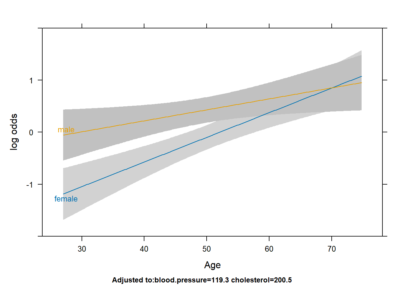
plot(Predict(fit2,cholesterol,sex))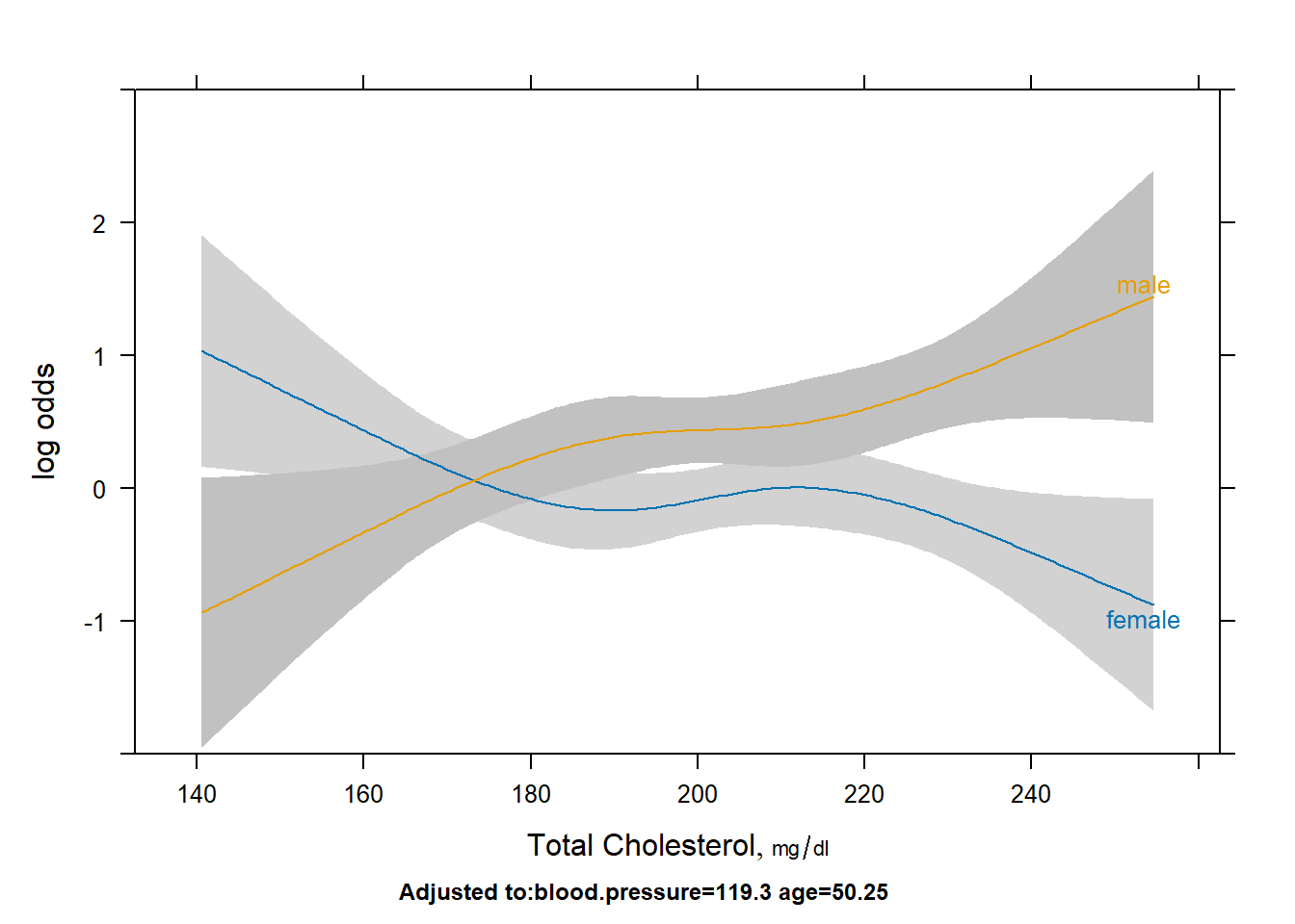
- We can use the non-overlapping confidence intervals to specify statistical significance. If this is too complicated we can also discuss the points where the lines cross. This is an open ended question.
- At ages below 50, the log odds of the outcome is statistically significantly higher for males compared to females. From ages 50 to 70, the log odds is still higher for males but the confidence intervals overlap so the difference is not as significant.
- For cholesterol levels below 150, the log odds of the outcome is statistically significantly higher for females compared to males. The opposite is true in cholesterol levels from 190 to 200, and above 220. There is a bit of overlap in confidence intervals between the 200-220 range.
# Fancy way of combining the plots together but is harder to interpret
bplot(Predict(fit2,cholesterol,age,sex,np=20),lfun=wireframe,drape=TRUE)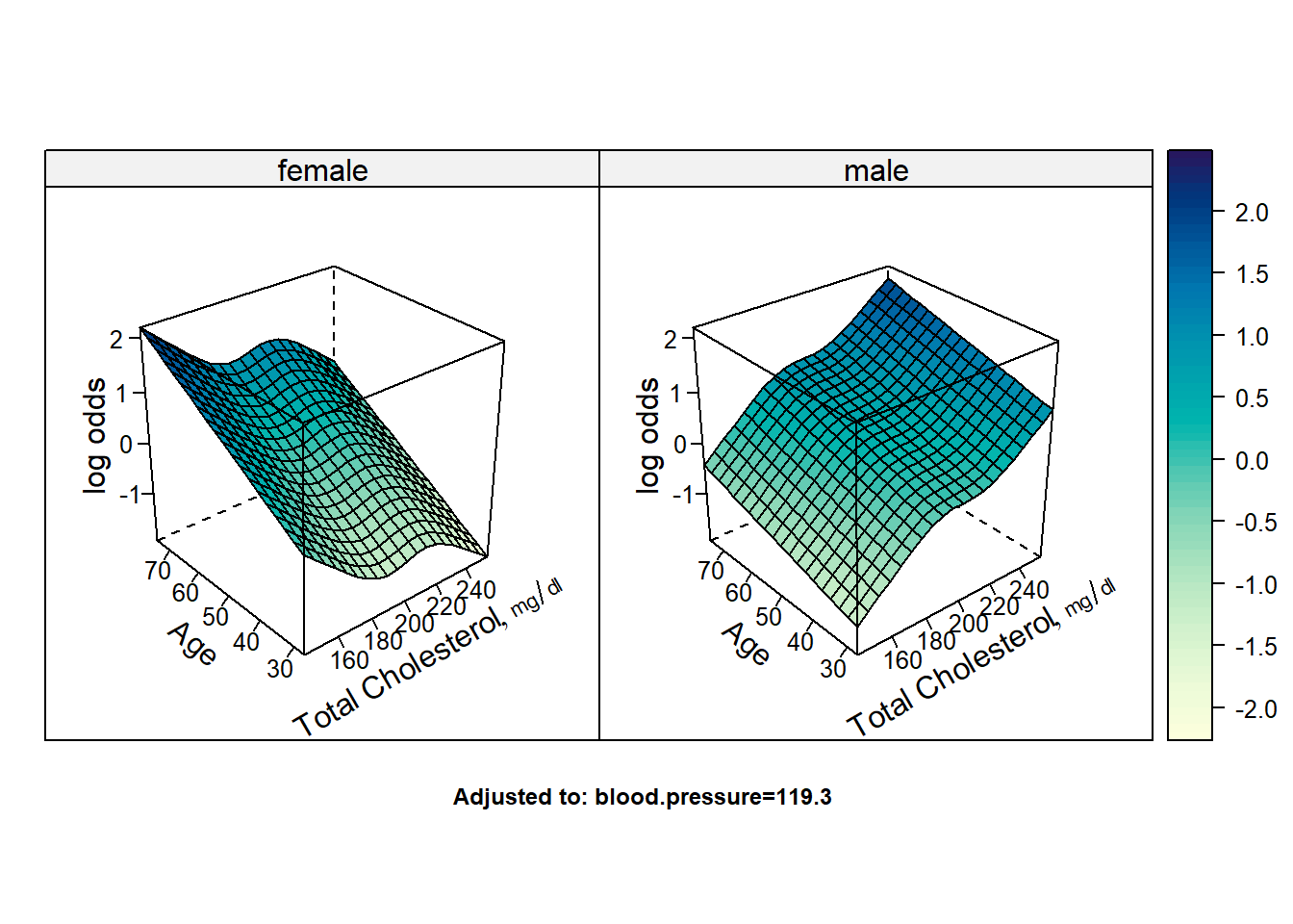
Extra
- Below we are fitting a third model with an interaction term between
sexand the other 3 variables, includingblood pressure.
fit3 <- lrm(y ~ sex * (blood.pressure + age + rcs(cholesterol,4)), data = tutdata)
# Alternate way
#lrm(y ~ sex + blood.pressure + age + rcs(cholesterol,4) + sex:blood.pressure + sex:age + sex:rcs(cholesterol,4), data = tutdata)

anova(fit3)
## Wald Statistics Response: y
##
## Factor Chi-Square d.f. P
## sex (Factor+Higher Order Factors) 39.12 6 <.0001
## All Interactions 26.58 5 0.0001
## blood.pressure (Factor+Higher Order Factors) 0.73 2 0.6954
## All Interactions 0.47 1 0.4940
## age (Factor+Higher Order Factors) 30.58 2 <.0001
## All Interactions 3.94 1 0.0471
## cholesterol (Factor+Higher Order Factors) 23.96 6 0.0005
## All Interactions 22.59 3 <.0001
## Nonlinear (Factor+Higher Order Factors) 5.24 4 0.2634
## sex * blood.pressure (Factor+Higher Order Factors) 0.47 1 0.4940
## sex * age (Factor+Higher Order Factors) 3.94 1 0.0471
## sex * cholesterol (Factor+Higher Order Factors) 22.59 3 <.0001
## Nonlinear 4.67 2 0.0966
## Nonlinear Interaction : f(A,B) vs. AB 4.67 2 0.0966
## TOTAL NONLINEAR 5.24 4 0.2634
## TOTAL INTERACTION 26.58 5 0.0001
## TOTAL NONLINEAR + INTERACTION 27.25 7 0.0003
## TOTAL 62.64 11 <.0001- The total interaction from the anova output is still statistically significant as it takes into account all interactions.
- We can also test for it below as follows:
lrtest(fit1,fit3)##
## Model 1: y ~ blood.pressure + sex + age + rcs(cholesterol, 4)
## Model 2: y ~ sex * (blood.pressure + age + rcs(cholesterol, 4))
##
## L.R. Chisq d.f. P
## 2.878410e+01 5.000000e+00 2.556193e-05- The sex and blood pressure interaction term from the anova output is not significant (p=0.494).
- This is equivalent to the p-value from the likelihood ratio test below:
lrtest(fit2,fit3)##
## Model 1: y ~ blood.pressure + sex * (age + rcs(cholesterol, 4))
## Model 2: y ~ sex * (blood.pressure + age + rcs(cholesterol, 4))
##
## L.R. Chisq d.f. P
## 0.4679391 1.0000000 0.4939368- Let’s try to plot the sex/blood pressure relationship:
plot(Predict(fit3,blood.pressure,sex))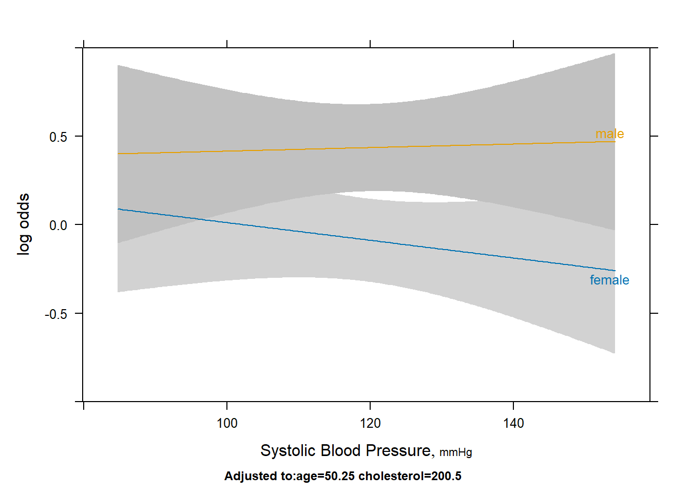
- At a first glance we do not see the lines meet like they do in the
sex:ageandsex:cholesterolinteractions. The confidence intervals also overlap for the most part, except in the 115-130 range. - Personally, I would avoid using this as a standalone method to check for a significant interaction, you should use either the anova function call or the likelihood ratio test.
Tutorial 5
Question 1
Using the data from the last few tutorials, fit the following model.
fit <- lrm(y ~ blood.pressure + sex * (age + rcs(cholesterol,4)), data = tutdata, x=TRUE, y=TRUE)
library(rms)
load("./CHL5202/tutdata.RData")

dd <- datadist(tutdata)
options(datadist = "dd")
fit <- lrm(y ~ blood.pressure + sex * (age + rcs(cholesterol, 4)), data = tutdata,
x = TRUE, y = TRUE)
fit## Logistic Regression Model
##
## lrm(formula = y ~ blood.pressure + sex * (age + rcs(cholesterol,
## 4)), data = tutdata, x = TRUE, y = TRUE)
##
## Model Likelihood Discrimination Rank Discrim.
## Ratio Test Indexes Indexes
## Obs 1000 LR chi2 69.39 R2 0.090 C 0.642
## 0 460 d.f. 10 R2(10,1000)0.058 Dxy 0.283
## 1 540 Pr(> chi2) <0.0001 R2(10,745.2)0.077 gamma 0.283
## max |deriv| 1e-08 Brier 0.232 tau-a 0.141
##
## Coef S.E. Wald Z Pr(>|Z|)
## Intercept 3.2474 2.3426 1.39 0.1657
## blood.pressure -0.0022 0.0044 -0.51 0.6105
## sex=male -9.3612 3.5422 -2.64 0.0082
## age 0.0474 0.0094 5.06 <0.0001
## cholesterol -0.0308 0.0133 -2.31 0.0209
## cholesterol' 0.0738 0.0376 1.96 0.0499
## cholesterol'' -0.3072 0.1552 -1.98 0.0477
## sex=male * age -0.0263 0.0134 -1.96 0.0495
## sex=male * cholesterol 0.0620 0.0203 3.06 0.0022
## sex=male * cholesterol' -0.1241 0.0569 -2.18 0.0293
## sex=male * cholesterol'' 0.5116 0.2362 2.17 0.0303Question 2
Validate the model using the bootstrap with 100 replications and comment on the overfitting.
set.seed(123)
validate(fit, B = 100)
## index.orig training test optimism index.corrected n
## Dxy 0.2832 0.3025 0.2685 0.0340 0.2493 100
## R2 0.0896 0.1024 0.0792 0.0232 0.0664 100
## Intercept 0.0000 0.0000 0.0108 -0.0108 0.0108 100
## Slope 1.0000 1.0000 0.8768 0.1232 0.8768 100
## Emax 0.0000 0.0000 0.0311 0.0311 0.0311 100
## D 0.0684 0.0788 0.0601 0.0187 0.0496 100
## U -0.0020 -0.0020 0.0013 -0.0033 0.0013 100
## Q 0.0704 0.0808 0.0588 0.0220 0.0484 100
## B 0.2316 0.2289 0.2341 -0.0052 0.2367 100
## g 0.6230 0.6708 0.5787 0.0921 0.5309 100
## gp 0.1457 0.1541 0.1358 0.0183 0.1273 100- There is mild evidence of overfitting.
- \(D_{xy}\) and Brier score
(
B) do not change much at all. - Slope parameter indicates a need to shrink by about 12% to calibrate
Question 3
Investigate influential observations and partial residual plots.
dff <- resid(fit, "dffits")
plot(dff)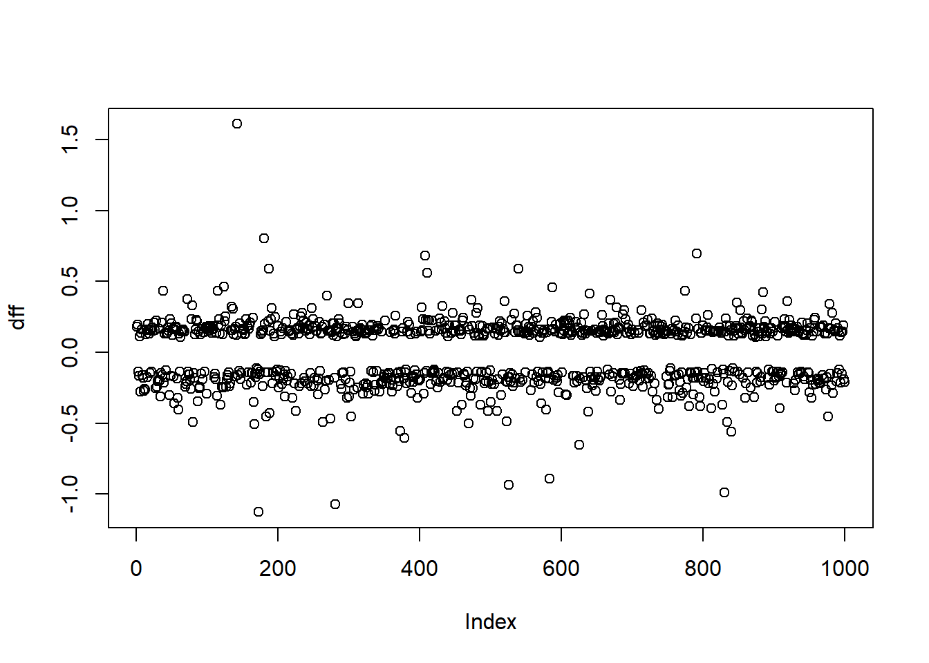
- The DFFITS statistic indicate the effect that deleting each observation has on the predicted values of the model.
- Some use \(|\text{DFFITS}| > 2\sqrt{\frac{p+1}{n-p-1}}\) to indicate an influential observation.
show.influence(which.influence(fit), data.frame(tutdata, dffits = dff), report = c("dffits"))## Count sex cholesterol dffits
## 143 2 female *274.0808 1.6108318
## 173 4 *female *138.5056 -1.1265158
## 181 2 *male 146.4978 0.8026558
## 408 2 *male 148.1649 0.6813596
## 411 1 female 146.3522 0.5594519
## 834 2 female *146.6413 -0.4908278
## 840 2 female *147.0025 -0.5604495- Using
which.influence()gives the indices of influential observations, which are listed in the first column of the dataframe above. - The variables with significant DFBETA are marked with an asterisk. Note that all of these observations have significant DFFITS.
- The DFBETAS are statistics that indicate the effect that deleting each observation has on the estimates for the regression coefficients.
- For DFBETAS one can use \(|\text{DFBETAS}| > u\) for a given cutoff, the default is 0.2.
Below we investigate partial residual plots which can be used to verify the functional form of continuous covariates.
# Option below saves the following plots to a pdf file
# pdf("resid_plots.pdf")

resid(fit, "partial", pl = "loess")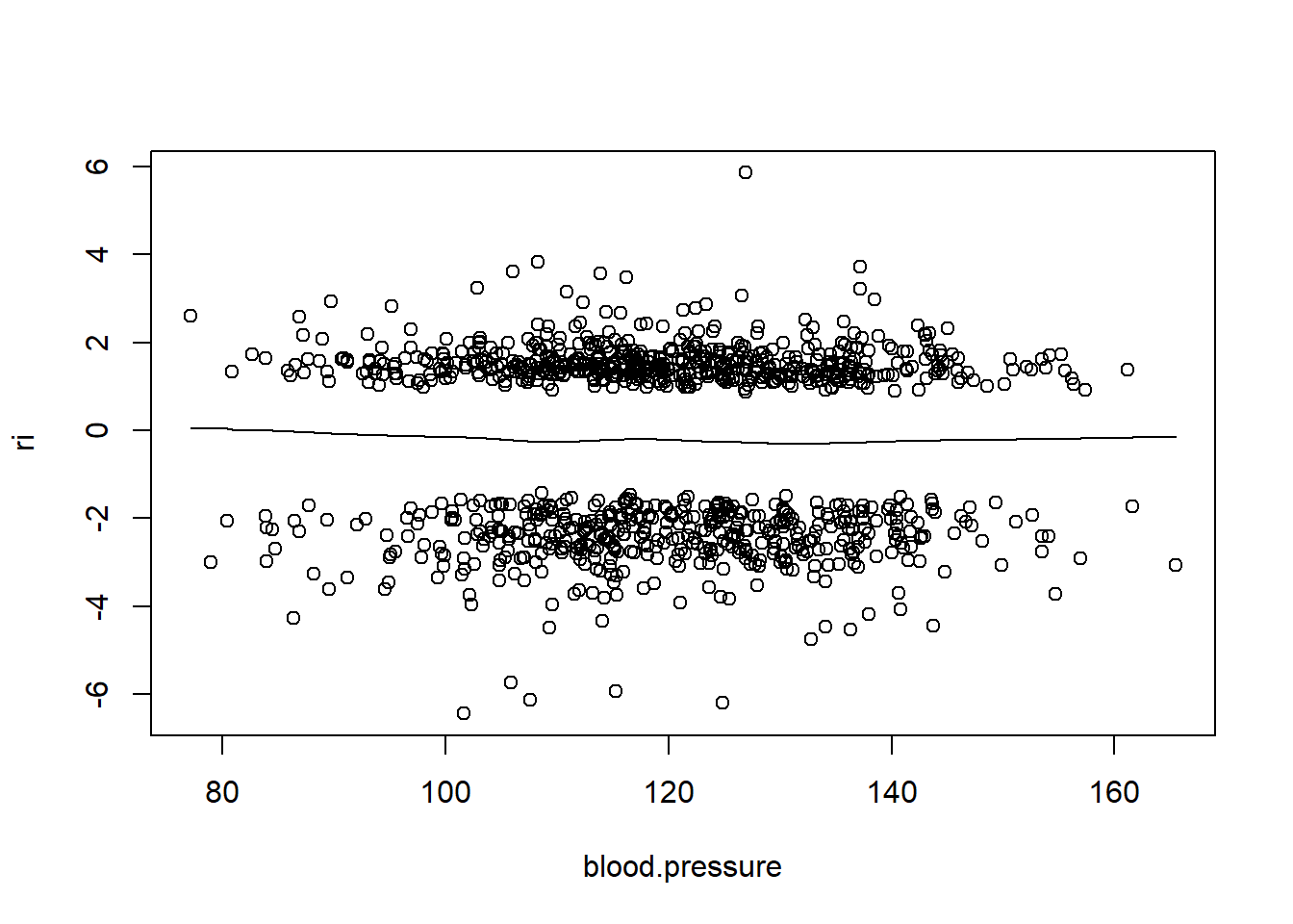
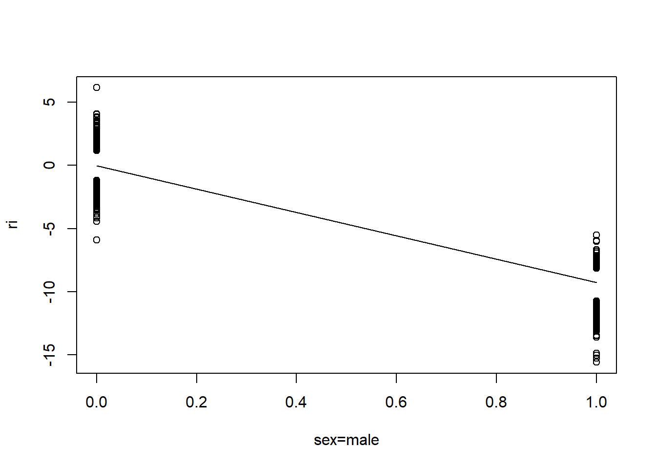
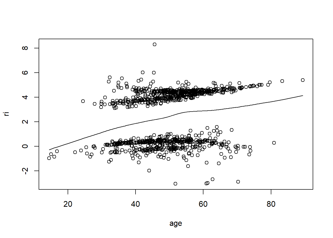
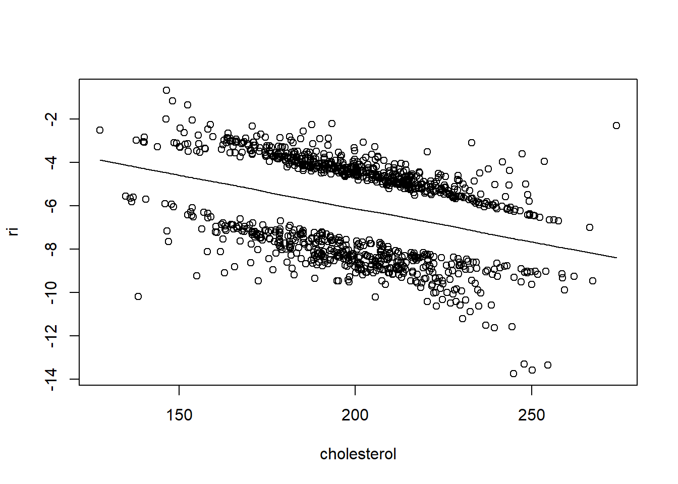
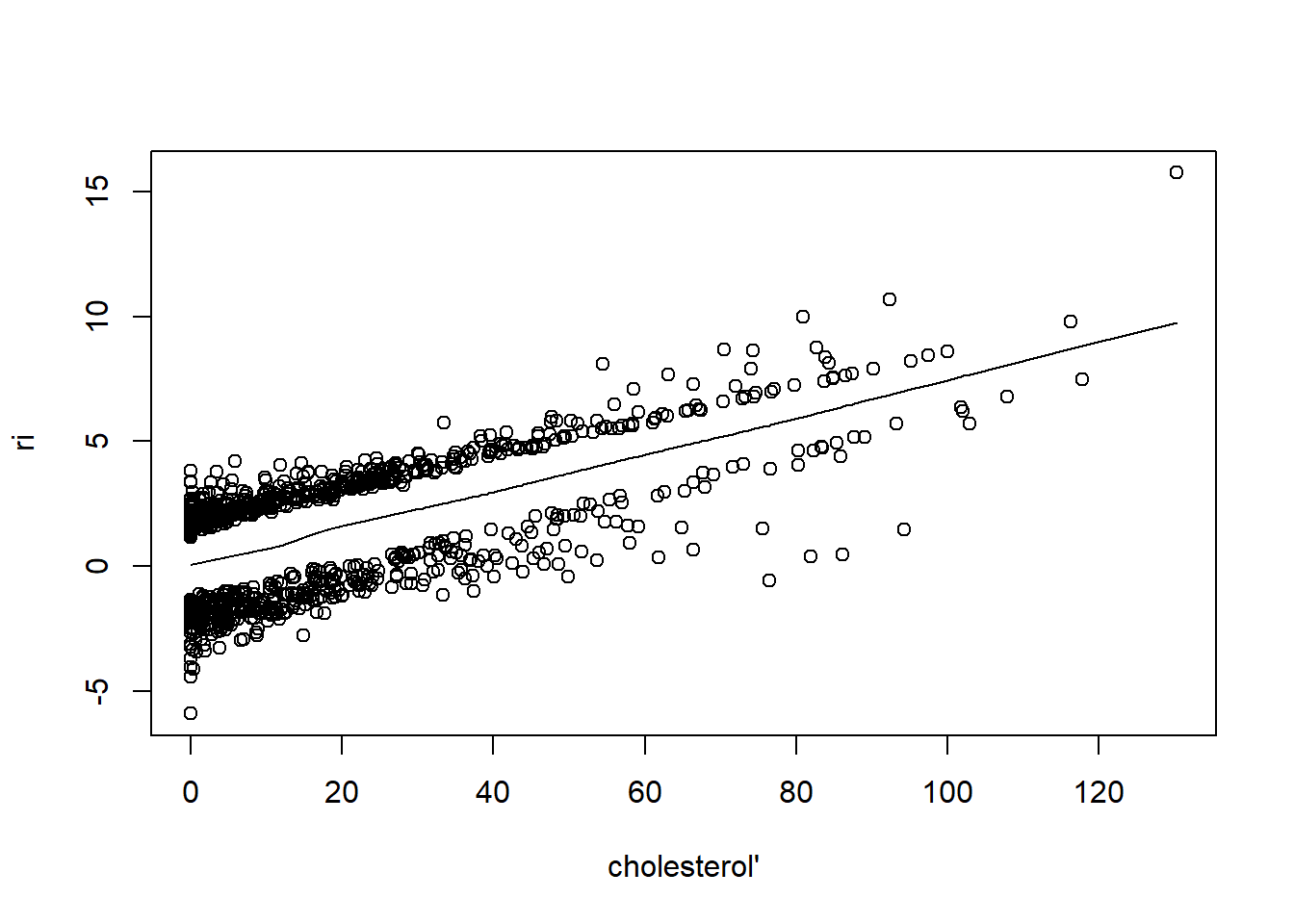
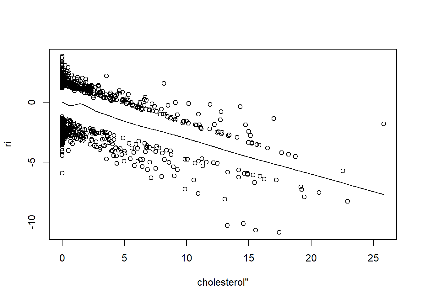
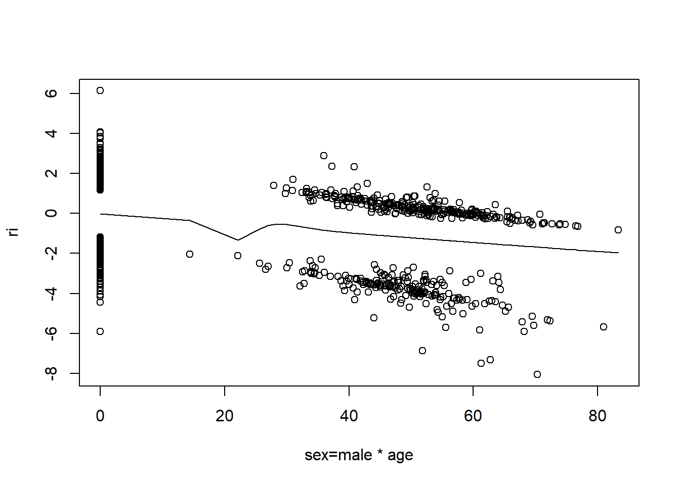
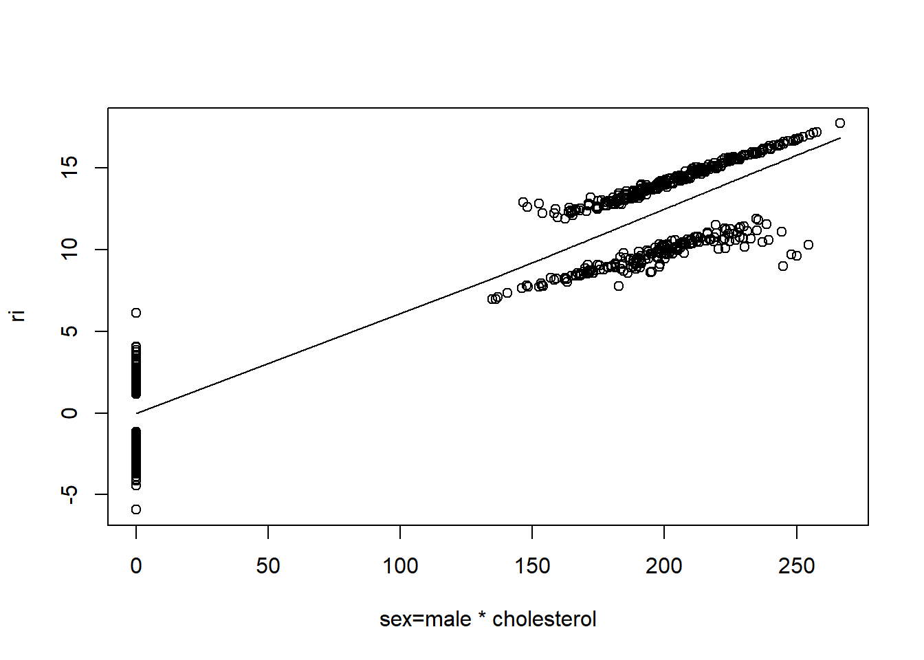
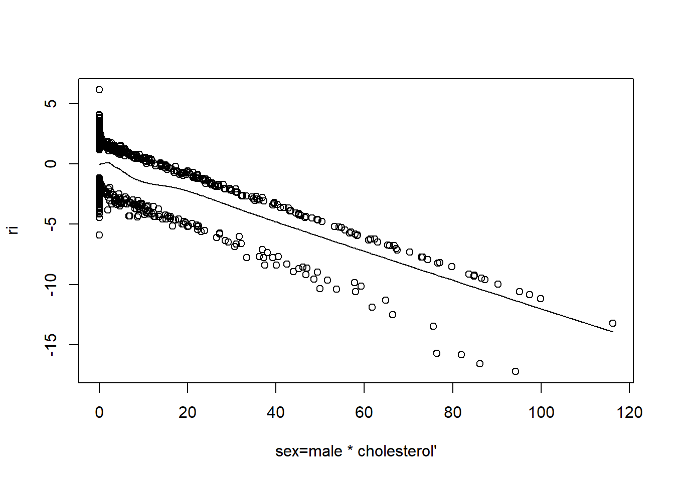
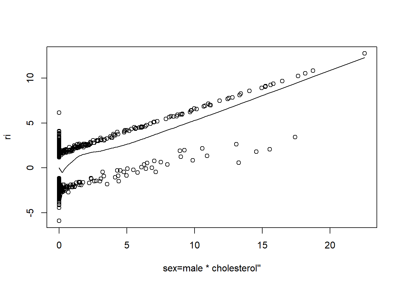
- There is very little evidence of non-linearity in most of these plots, i.e. there is not much value in including a non-linear component for these variables.
Tutorial 6
Over the next few weeks the tutorials will use the data frame
mgus2 which may be found in the survival package. Since the
survival package is attached when rms is, nothing special
is required to access it, other than loading the rms
package. Update: it needs to be loaded from the survival
package.
library(rms)
library(survival)

str(mgus2)
## 'data.frame': 1384 obs. of 11 variables:
## $ id : num 1 2 3 4 5 6 7 8 9 10 ...
## $ age : num 88 78 94 68 90 90 89 87 86 79 ...
## ..- attr(*, "label")= chr "AGE AT mgus_sp"
## $ sex : Factor w/ 2 levels "F","M": 1 1 2 2 1 2 1 1 1 1 ...
## ..- attr(*, "label")= chr "Sex"
## ..- attr(*, "format")= chr "$desex"
## $ dxyr : num 1981 1968 1980 1977 1973 ...
## $ hgb : num 13.1 11.5 10.5 15.2 10.7 12.9 10.5 12.3 14.5 9.4 ...
## $ creat : num 1.3 1.2 1.5 1.2 0.8 1 0.9 1.2 0.9 1.1 ...
## $ mspike: num 0.5 2 2.6 1.2 1 0.5 1.3 1.6 2.4 2.3 ...
## ..- attr(*, "label")= chr "SEP SPIKE AT mgus_sp"
## $ ptime : num 30 25 46 92 8 4 151 2 57 136 ...
## $ pstat : num 0 0 0 0 0 0 0 0 0 0 ...
## $ futime: num 30 25 46 92 8 4 151 2 57 136 ...
## $ death : num 1 1 1 1 1 1 1 1 0 1 ...More information about the data can be found in the help file
(e.g. ?mgus2).
Question 1
Estimate the Kaplan-Meier curves for survival for males and females and plot the result.
# The rms package has a function npsurv which is used in place of the usual survfit.
fit <- npsurv(Surv(futime, death) ~ sex, data = mgus2)

# Two methods below:
plot(fit, lty = c(1, 2)) # standard method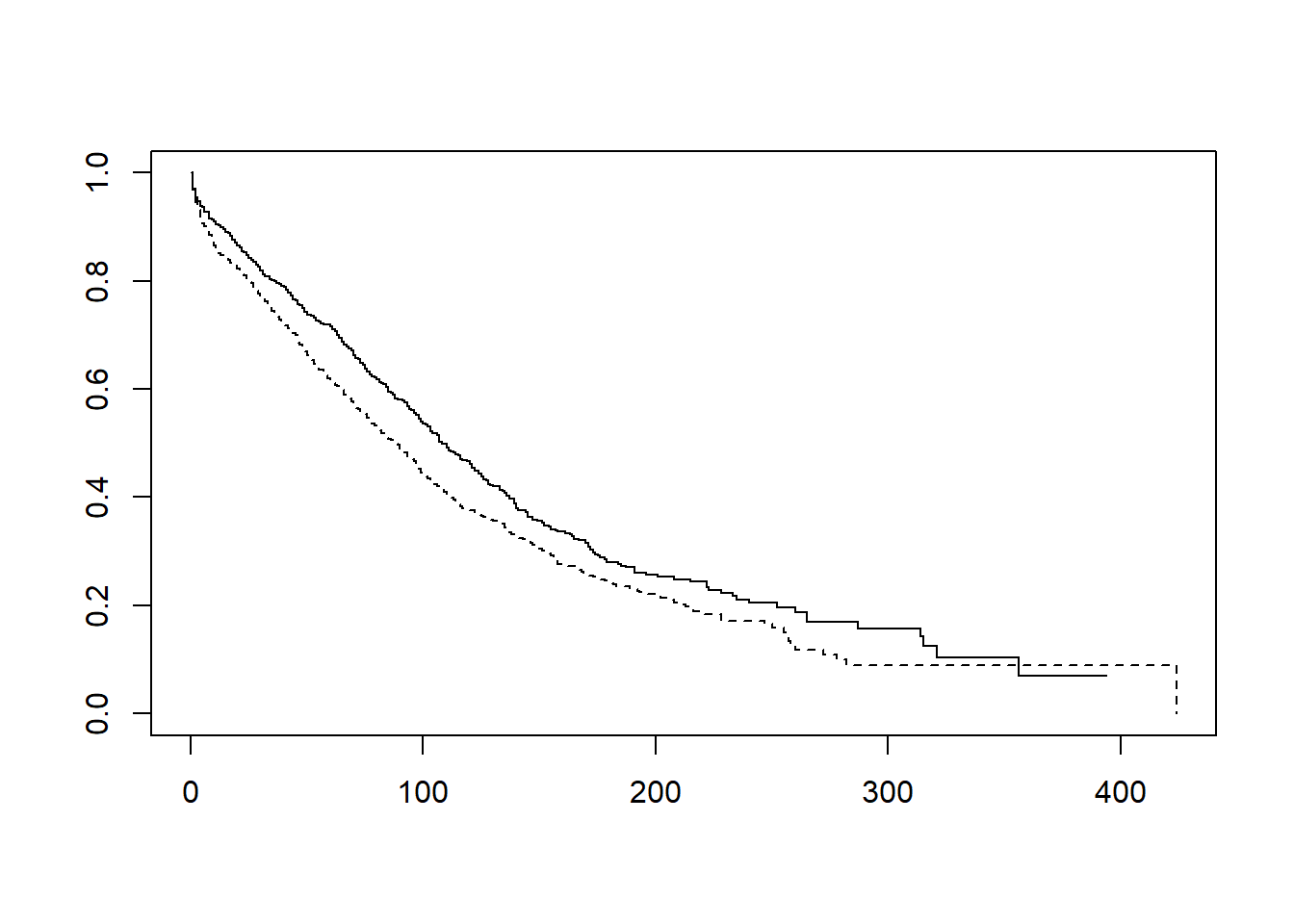
survplot(fit, n.risk = TRUE) #a more flexible function from rms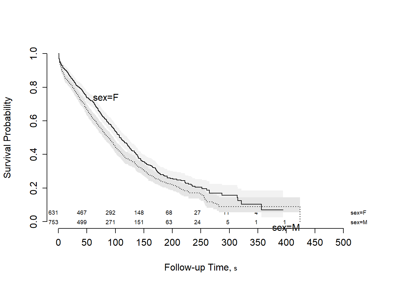
Question 2
Test \(H_0 : S_F(t) = S_M(t)\) versus \(H_0 : S_F(t) \neq S_M(t).\)
# This requires the Mantel-Haenzel (log-rank) test.
print(fit.mh <- survdiff(Surv(futime, death) ~ sex, data = mgus2))
## Call:
## survdiff(formula = Surv(futime, death) ~ sex, data = mgus2)
##
## N Observed Expected (O-E)^2/E (O-E)^2/V
## sex=F 631 423 471 4.88 9.67
## sex=M 753 540 492 4.67 9.67
##
## Chisq= 9.7 on 1 degrees of freedom, p= 0.002- The Mantel-Haenzel test yields a p-value of 0.002, so we reject the null hypothesis as there is strong evidence that the survival function for females is not equal to the survival function for males.
Question 3
Compute the risk difference at one year.
(summ <- summary(fit, times = 12)) # time is in months## Call: npsurv(formula = Surv(futime, death) ~ sex, data = mgus2)
##
## sex=F
## time n.risk n.event survival std.err lower 95% CI
## 12.0000 569.0000 61.0000 0.9032 0.0118 0.8804
## upper 95% CI
## 0.9266
##
## sex=M
## time n.risk n.event survival std.err lower 95% CI
## 12.000 646.000 112.000 0.851 0.013 0.826
## upper 95% CI
## 0.877- The risk difference (assigning females as control and males as treatment) is:
\[ \begin{aligned} \widehat{RD} &= \hat{F}_C(t_0)-\hat{F}_T(t_0) \\ &= (1-\hat{S}_C(t_0))(1-\hat{S}_T(t_0)) \\ &= \hat{S}_T(t_0)-\hat{S}_C(t_0) \\ &= 0.851 - 0.9032 \\ &= -0.0522 \end{aligned} \]
- Using R:
(rd <- summ$surv[2] - summ$surv[1])## [1] -0.05194881fit$surv[length(fit$surv)-232+12] - fit$surv[12] # alternative## [1] -0.05194881Interpretation: The observed risk of death in females at one year is 5.2% lower than in males.
(Extra) A 95% confidence interval for the risk difference is:
\[ \begin{aligned} &\widehat{RD} \pm 1.96\sqrt{\hat{V}[\hat{S}_C(t_0)] + \hat{V}[\hat{S}_T(t_0)]} \\ &= -0.0522 \pm 1.96\sqrt{0.0118^2 + 0.013^2} \\ &= (-0.0866,-0.0178) \end{aligned} \]
- Using R:
bound <- 1.96*sqrt(summ$std.err[1]^2 + summ$std.err[2]^2)

c(rd-bound, rd+bound)
## [1] -0.08628336 -0.01761427Question 4
Compute a hazard ratio using the output from
survdiff.
\[ \widehat{HR} = \frac{O_T/E_T}{O_C/E_C} = \frac{540/492}{423/471} = 1.222 \]
- Alternatively, we can calculate using
fit.mh:
# We can extract the numbers from fit.mh
fit.mh$obs
## [1] 423 540fit.mh$exp## [1] 470.9283 492.0717# Observed / Expected
female <- fit.mh$obs[1]/fit.mh$exp[1] # 423/471
male <- fit.mh$obs[2]/fit.mh$exp[2] # 540/492
# Hazard Ratio Using females as reference
hr <- male/female # (540/492)/(423/471)
hr## [1] 1.221743The hazard ratio of 1.222 means that the rate of death for males is 1.222 times the rate of death for females.
(Extra) Obtaining a 95% CI for the hazard ratio, we start with the standard error:
\[ SE[\log\widehat{HR}] = \sqrt{\frac{1}{E_T} + \frac{1}{E_C}} = \sqrt{\frac{1}{492} + \frac{1}{471}} = 0.06446 \]
- Which gives a 95% CI of:
\[ 1.222 \times e^{\pm1.96\times0.06446} = (1.0769,1.3866) \]
- Using R:
# Standard error of log hazard ratio
se <- sqrt((1/fit.mh$exp[2]) + (1/fit.mh$exp[1]))

# 95% Confidence interval
c(1.222*exp(-1.96*se), 1.222*exp(+1.96*se))
## [1] 1.076956 1.386579Tutorial 7
You will again use the data frame mgus2 from the
rms package.
library(rms)

str(mgus2)
## 'data.frame': 1384 obs. of 11 variables:
## $ id : num 1 2 3 4 5 6 7 8 9 10 ...
## $ age : num 88 78 94 68 90 90 89 87 86 79 ...
## ..- attr(*, "label")= chr "AGE AT mgus_sp"
## $ sex : Factor w/ 2 levels "F","M": 1 1 2 2 1 2 1 1 1 1 ...
## ..- attr(*, "label")= chr "Sex"
## ..- attr(*, "format")= chr "$desex"
## $ dxyr : num 1981 1968 1980 1977 1973 ...
## $ hgb : num 13.1 11.5 10.5 15.2 10.7 12.9 10.5 12.3 14.5 9.4 ...
## $ creat : num 1.3 1.2 1.5 1.2 0.8 1 0.9 1.2 0.9 1.1 ...
## $ mspike: num 0.5 2 2.6 1.2 1 0.5 1.3 1.6 2.4 2.3 ...
## ..- attr(*, "label")= chr "SEP SPIKE AT mgus_sp"
## $ ptime : num 30 25 46 92 8 4 151 2 57 136 ...
## $ pstat : num 0 0 0 0 0 0 0 0 0 0 ...
## $ futime: num 30 25 46 92 8 4 151 2 57 136 ...
## $ death : num 1 1 1 1 1 1 1 1 0 1 ...dd <- datadist(mgus2)
options(datadist = "dd")Question 1
Investigate if either the exponential or Weibull models would be appropriate to model the dependency of survival on sex.
fit.km <- npsurv(Surv(futime, death) ~ sex, data = mgus2)

# Check exponential
plot(fit.km, fun = "cumhaz")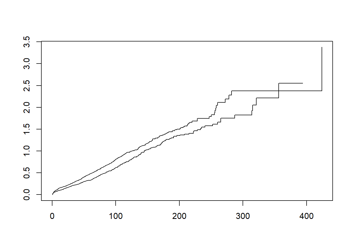
# Check Weibull
plot(fit.km, fun = "cloglog")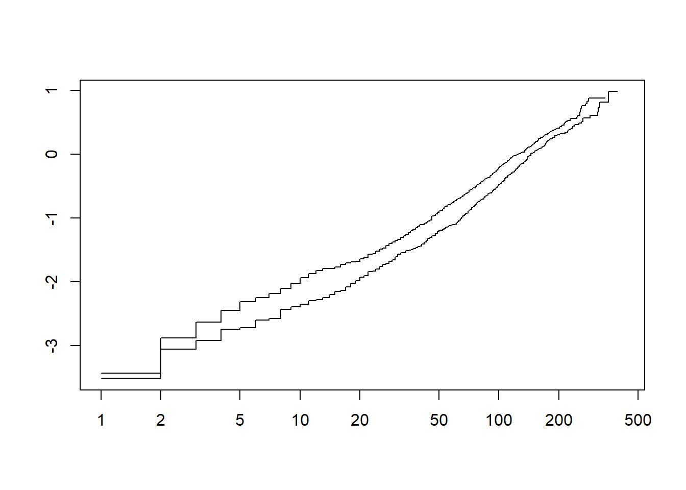
- The plots indicate that both models could be a good fit (as they are linear).
Question 2
Fit and interpret an exponential model and plot the result.
print(fit1 <- psm(Surv(futime,death)~sex,data=mgus2,dist="exponential"))## Parametric Survival Model: Exponential Distribution
##
## psm(formula = Surv(futime, death) ~ sex, data = mgus2, dist = "exponential")
##
## Model Likelihood Discrimination
## Ratio Test Indexes
## Obs 1384 LR chi2 9.99 R2 0.007
## Events 963 d.f. 1 R2(1,1384)0.006
## sigma 1.0000 Pr(> chi2) 0.0016 R2(1,963)0.009
## Dxy 0.062
##
## Coef S.E. Wald Z Pr(>|Z|)
## (Intercept) 5.0344 0.0486 103.54 <0.0001
## sex=M -0.2045 0.0649 -3.15 0.0016- P-value of 0.0016 provides strong evidence that the rate of death is higher in males than females.
# HR for sex: M vs. F
exp(-coef(fit1)[2])
## sex=M
## 1.226934- The hazard ratio of 1.227 means that the rate of death for males is 1.227 times the rate of death for females.
# Survival time ratio
summary(fit1,sex="F")
## Effects Response : Surv(futime, death)
##
## Factor Low High Diff. Effect S.E. Lower 0.95 Upper 0.95
## sex - M:F 1 2 NA -0.20452 0.06493 -0.33189 -0.077146
## Survival Time Ratio 1 2 NA 0.81504 NA 0.71757 0.925750- The survival time ratio of 0.815 means that the median survival time for males is 0.815 times the median survival time for females.
- The results can be interpreted in terms of any percentile survival time, but median is most common.
- For the exponential model, the survival time ratio is the inverse of the hazard ratio. This is not the case for other models.
survplot(fit1,sex)
survplot(fit.km,add=TRUE,label.curves=FALSE,conf="none",col="red")
Question 3
Fit and interpret a Weibull model and plot the result.
print(fit2 <- psm(Surv(futime,death)~sex,data=mgus2,dist="weibull"))## Parametric Survival Model: Weibull Distribution
##
## psm(formula = Surv(futime, death) ~ sex, data = mgus2, dist = "weibull")
##
## Model Likelihood Discrimination
## Ratio Test Indexes
## Obs 1384 LR chi2 9.18 R2 0.007
## Events 963 d.f. 1 R2(1,1384)0.006
## sigma 1.1016 Pr(> chi2) 0.0024 R2(1,963)0.008
## Dxy 0.062
##
## Coef S.E. Wald Z Pr(>|Z|)
## (Intercept) 5.0494 0.0538 93.87 <0.0001
## sex=M -0.2162 0.0716 -3.02 0.0025
## Log(scale) 0.0967 0.0278 3.48 0.0005- P-value of 0.0025 provides strong evidence that the rate of death is higher in males than females.
# HR for sex: M vs. F
exp(-coef(fit2)[2]/fit2$scale)
## sex=M
## 1.216865- The rate of death for males is 1.217 times the rate of death for females.
# Survival time ratio
summary(fit2,sex="F")
## Effects Response : Surv(futime, death)
##
## Factor Low High Diff. Effect S.E. Lower 0.95 Upper 0.95
## sex - M:F 1 2 NA -0.21622 0.071609 -0.35669 -0.075742
## Survival Time Ratio 1 2 NA 0.80556 NA 0.69999 0.927060- The median survival time for males is 0.806 times the median survival time for females.
survplot(fit2,sex)
survplot(fit.km,add=TRUE,label.curves=FALSE,conf="none",col="red")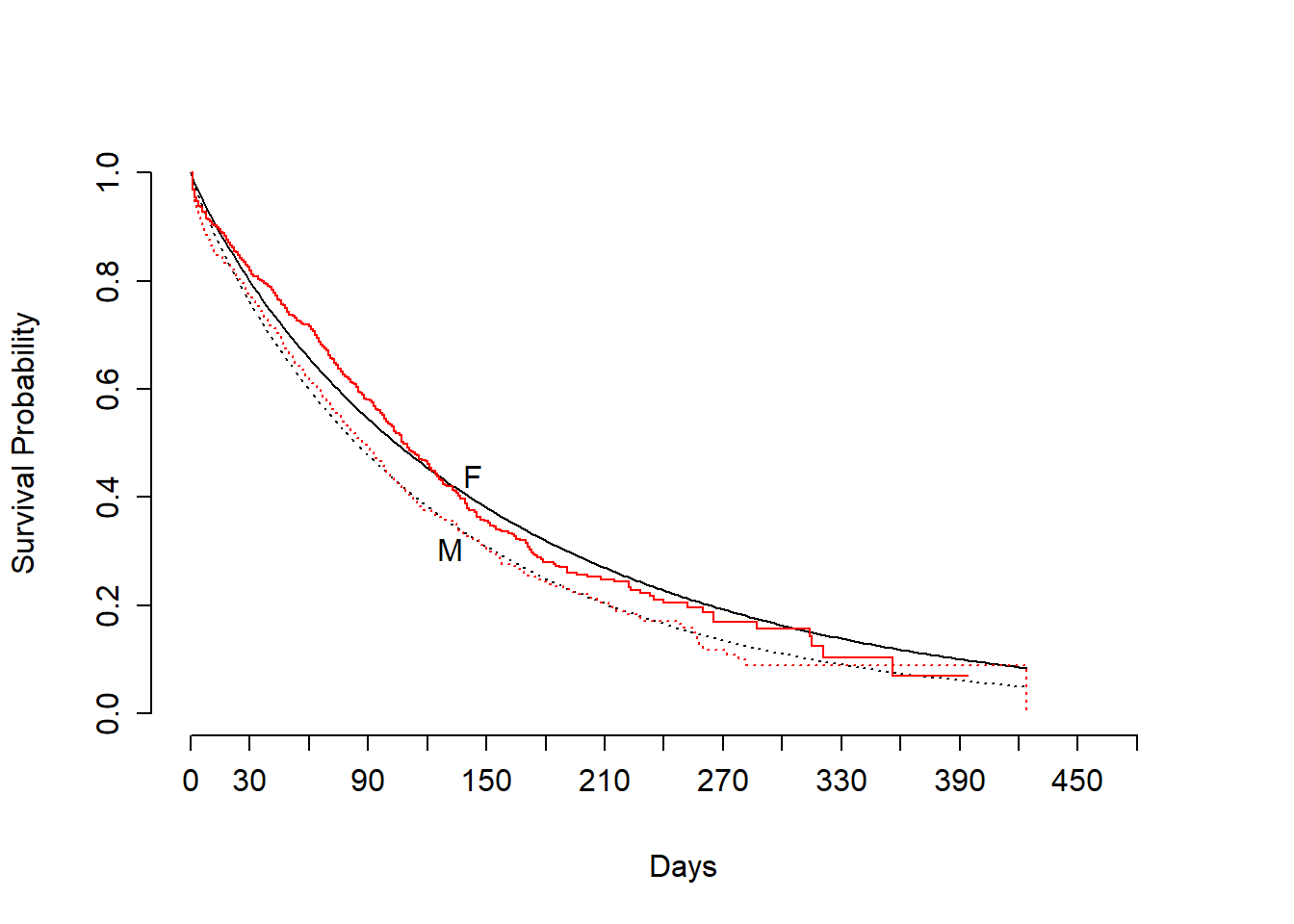
Question 4
Which looks better (exponential or Weibull)?
survplot(fit.km,conf="none")
survplot(fit1,sex,add=TRUE,label.curves=FALSE,col="red") # exponential
survplot(fit2,sex,add=TRUE,label.curves=FALSE,col="blue") # weibull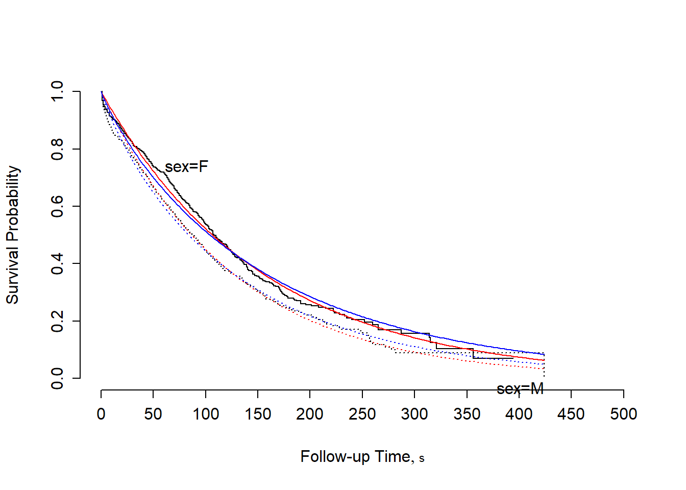
- There’s very little difference between the two models in this example. The AIC for the Weibull is slightly smaller, which may or may not mean anything.
Question 5
Fit a Cox model with sex as the covariate and interpret.
print(fit1.cox <- cph(Surv(futime,death)~sex,data=mgus2))## Cox Proportional Hazards Model
##
## cph(formula = Surv(futime, death) ~ sex, data = mgus2)
##
## Model Tests Discrimination
## Indexes
## Obs 1384 LR chi2 9.68 R2 0.007
## Events 963 d.f. 1 R2(1,1384)0.006
## Center 0.1098 Pr(> chi2) 0.0019 R2(1,963)0.009
## Score chi2 9.65 Dxy 0.062
## Pr(> chi2) 0.0019
##
## Coef S.E. Wald Z Pr(>|Z|)
## sex=M 0.2017 0.0651 3.10 0.0019summary(fit1.cox,sex="F")## Effects Response : Surv(futime, death)
##
## Factor Low High Diff. Effect S.E. Lower 0.95 Upper 0.95
## sex - M:F 1 2 NA 0.20174 0.065062 0.074221 0.32926
## Hazard Ratio 1 2 NA 1.22350 NA 1.077000 1.38990- The rate of death for males is 1.224 times the rate of death for females.
- There is strong evidence that the rate of death is higher in males than females (HR=1.22350; 95% CI: (1.07700,1.38990); p-value: 0.0019)
Question 6
Add age using a restricted cubic spline with 4 knots. Test it with a LRT and display results.
print(fit2.cox <- cph(Surv(futime,death)~sex+rcs(age,4),data=mgus2))## Cox Proportional Hazards Model
##
## cph(formula = Surv(futime, death) ~ sex + rcs(age, 4), data = mgus2)
##
## Model Tests Discrimination
## Indexes
## Obs 1384 LR chi2 396.10 R2 0.249
## Events 963 d.f. 4 R2(4,1384)0.247
## Center 3.248 Pr(> chi2) 0.0000 R2(4,963)0.334
## Score chi2 408.99 Dxy 0.334
## Pr(> chi2) 0.0000
##
## Coef S.E. Wald Z Pr(>|Z|)
## sex=M 0.3605 0.0657 5.48 <0.0001
## age 0.0380 0.0108 3.52 0.0004
## age' 0.0473 0.0214 2.21 0.0272
## age'' -0.2396 0.1233 -1.94 0.0520# LRT
lrtest(fit1.cox,fit2.cox)##
## Model 1: Surv(futime, death) ~ sex
## Model 2: Surv(futime, death) ~ sex + rcs(age, 4)
##
## L.R. Chisq d.f. P
## 386.42 3.00 0.00- We are testing the null hypothesis that the coefficients for the age variable are equal to 0, against the alternative hypothesis that at least one coefficient is not equal to 0.
- Since the p-value is approximately 0.00, there is sufficient evidence to suggest that we should retain the age variable using a restricted cubic spline with 4 knots.
# Adjusted effect for sex
summary(fit2.cox,sex="F")
## Effects Response : Surv(futime, death)
##
## Factor Low High Diff. Effect S.E. Lower 0.95 Upper 0.95
## age 63 79 16 1.13420 0.094988 0.94802 1.32040
## Hazard Ratio 63 79 16 3.10870 NA 2.58060 3.74480
## sex - M:F 1 2 NA 0.36049 0.065742 0.23164 0.48935
## Hazard Ratio 1 2 NA 1.43400 NA 1.26070 1.63120- The rate of death for 79-year-olds is 3.109 times the rate of death
for 63-year-olds when adjusted for
sex. - There is strong evidence that the rate of death is higher in 79-year-olds than 63-year-olds (HR=3.10870; 95% CI: (2.58060,3.74480), p-value: 0.0004)
- The rate of death for males is 1.434 times the rate of death for
females when adjusted for
age. - There is strong evidence that the rate of death is higher in males than females (HR=1.43400; 95% CI: (1.26070,1.63120); p-value: <0.0001)
# You can specify the specific age groups
summary(fit2.cox,sex="F",age=c(40,80))
## Effects Response : Surv(futime, death)
##
## Factor Low High Diff. Effect S.E. Lower 0.95 Upper 0.95
## age 40 80 40 2.16870 0.194200 1.78810 2.54930
## Hazard Ratio 40 80 40 8.74700 NA 5.97800 12.79800
## sex - M:F 1 2 NA 0.36049 0.065742 0.23164 0.48935
## Hazard Ratio 1 2 NA 1.43400 NA 1.26070 1.63120- The rate of death for 80-year-olds is 8.747 times the rate of death for 40-year-olds.
- Note that the hazard ratio for
sexremains unchanged.
# Plot of age effect
plot(Predict(fit2.cox,age,sex))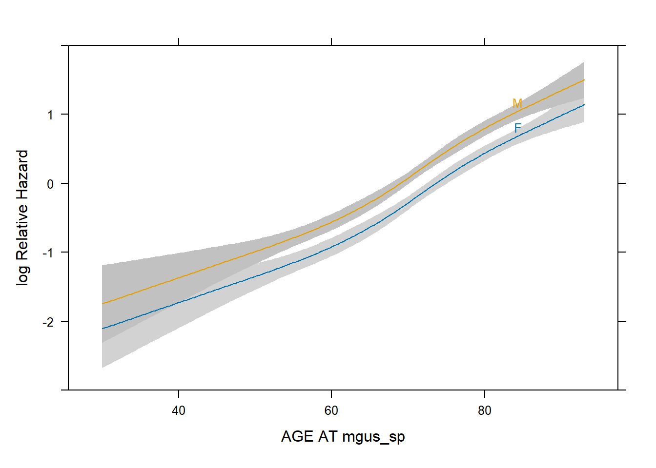
- The vertical distance between the two curves remain constant
throughout as that represents the
sexeffect. - The curves both fluctuate together depending on the
age.
Tutorial 8
You will again use the data frame mgus2 from the
rms package.
library(rms)

str(mgus2)
## 'data.frame': 1384 obs. of 11 variables:
## $ id : num 1 2 3 4 5 6 7 8 9 10 ...
## $ age : num 88 78 94 68 90 90 89 87 86 79 ...
## ..- attr(*, "label")= chr "AGE AT mgus_sp"
## $ sex : Factor w/ 2 levels "F","M": 1 1 2 2 1 2 1 1 1 1 ...
## ..- attr(*, "label")= chr "Sex"
## ..- attr(*, "format")= chr "$desex"
## $ dxyr : num 1981 1968 1980 1977 1973 ...
## $ hgb : num 13.1 11.5 10.5 15.2 10.7 12.9 10.5 12.3 14.5 9.4 ...
## $ creat : num 1.3 1.2 1.5 1.2 0.8 1 0.9 1.2 0.9 1.1 ...
## $ mspike: num 0.5 2 2.6 1.2 1 0.5 1.3 1.6 2.4 2.3 ...
## ..- attr(*, "label")= chr "SEP SPIKE AT mgus_sp"
## $ ptime : num 30 25 46 92 8 4 151 2 57 136 ...
## $ pstat : num 0 0 0 0 0 0 0 0 0 0 ...
## $ futime: num 30 25 46 92 8 4 151 2 57 136 ...
## $ death : num 1 1 1 1 1 1 1 1 0 1 ...dd <- datadist(mgus2)
options(datadist = "dd")Question 1
Fit a Cox model with sex as the only covariate and test
the proportional hazards assumption.
fit1 <- cph(Surv(futime, death) ~ sex, data = mgus2, x = TRUE, y = TRUE)
print(fit1.zph <- cox.zph(fit1))
## chisq df p
## sex 2.47 1 0.12
## GLOBAL 2.47 1 0.12# scaled Schoenfeld residuals
plot(fit1.zph)
abline(h=coef(fit1)[1], col="red", lwd=2, lty=3)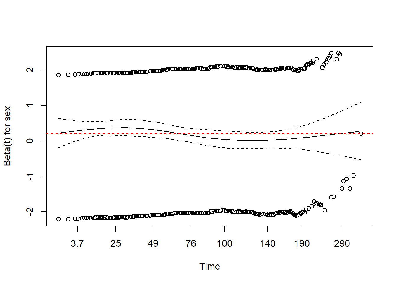
- If the proportional hazards assumption for \(x_j\) is true, a plot of scaled Schoenfeld residuals versus time should be a horizontal line at \(\hat{\beta}\).
- In this case the (red) line is not perfectly horizontal however it falls within the 95% confidence interval, meaning that the proportional hazards assumption is satisfied.
Question 2
Estimate a suitable transformation of hgb after
adjustment for sex.
res <- resid(fit1)
res.lo <- loess(res ~ hgb, data = mgus2)
# restricted cubic spline with 5 knots
res.ols <- ols(res ~ rcs(hgb, 5), data = mgus2)

plot(Predict(res.ols, hgb), addpanel = function(...) {
  panel.points(mgus2$hgb, res)
  panel.lines(seq(5, 20, length.out = 25),
              predict(res.lo, seq(5, 20, length.out = 25)),
              col = "red")
}, ylim = 1.15 * range(res), ylab = "Martingale Residual", xlab = "Hgb")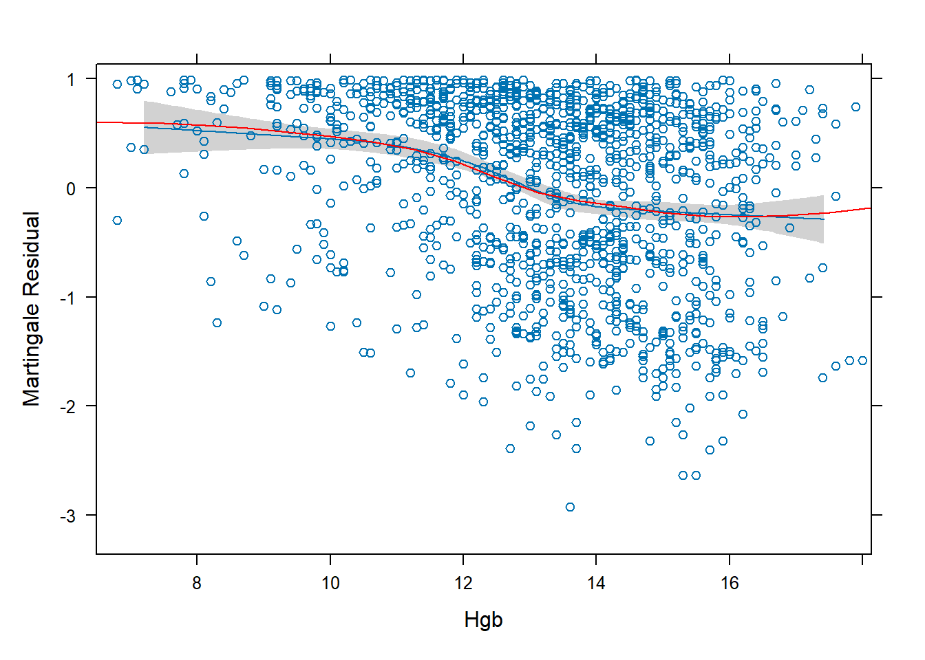
- This plot of the Martingale Residuals suggests a restricted cubic spline with 5 knots is reasonable.
- The number of knots was decided by trial and error – the blue line did not align with the red line when using numbers other than 5.
Question 3
Fit a Cox model that includes sex, hgb,
creat and age. Model the continuous variables
with 5 knot splines and include interactions between sex
and the other variables. Validate the model for overfitting.
fit2 <- cph(Surv(futime, death) ~ sex * (rcs(age, 5) + rcs(hgb, 5) + rcs(creat,5)),
            data = mgus2, x = TRUE, y = TRUE)
anova(fit2)
## Wald Statistics Response: Surv(futime, death)
##
## Factor Chi-Square d.f. P
## sex (Factor+Higher Order Factors) 40.49 13 0.0001
## All Interactions 14.79 12 0.2529
## age (Factor+Higher Order Factors) 251.27 8 <.0001
## All Interactions 0.27 4 0.9919
## Nonlinear (Factor+Higher Order Factors) 7.46 6 0.2805
## hgb (Factor+Higher Order Factors) 56.74 8 <.0001
## All Interactions 0.36 4 0.9859
## Nonlinear (Factor+Higher Order Factors) 12.45 6 0.0527
## creat (Factor+Higher Order Factors) 44.76 8 <.0001
## All Interactions 13.57 4 0.0088
## Nonlinear (Factor+Higher Order Factors) 28.66 6 0.0001
## sex * age (Factor+Higher Order Factors) 0.27 4 0.9919
## Nonlinear 0.23 3 0.9718
## Nonlinear Interaction : f(A,B) vs. AB 0.23 3 0.9718
## sex * hgb (Factor+Higher Order Factors) 0.36 4 0.9859
## Nonlinear 0.08 3 0.9945
## Nonlinear Interaction : f(A,B) vs. AB 0.08 3 0.9945
## sex * creat (Factor+Higher Order Factors) 13.57 4 0.0088
## Nonlinear 11.36 3 0.0100
## Nonlinear Interaction : f(A,B) vs. AB 11.36 3 0.0100
## TOTAL NONLINEAR 48.33 18 0.0001
## TOTAL INTERACTION 14.79 12 0.2529
## TOTAL NONLINEAR + INTERACTION 56.21 21 <.0001
## TOTAL 468.25 25 <.0001set.seed(1)
validate(fit2,B=100)## Warning in fitter(..., strata = strata, rownames = rownames, offset = offset, :
## Loglik converged before variable 24 ; coefficient may be infinite.## Warning in fitter(..., strata = strata, rownames = rownames, offset = offset, :
## Loglik converged before variable 15 ; coefficient may be infinite.## Warning in fitter(..., strata = strata, rownames = rownames, offset = offset, :
## Loglik converged before variable 18 ; coefficient may be infinite.## index.orig training test optimism index.corrected n
## Dxy 0.4023 0.4112 0.3951 0.0162 0.3862 100
## R2 0.3091 0.3220 0.2878 0.0342 0.2749 100
## Slope 1.0000 1.0000 0.8882 0.1118 0.8882 100
## D 0.0407 0.0428 0.0374 0.0054 0.0353 100
## U -0.0002 -0.0002 0.0021 -0.0023 0.0021 100
## Q 0.0408 0.0429 0.0352 0.0077 0.0331 100
## g 0.9390 0.9708 0.8629 0.1079 0.8312 100- The warning produced indicates that on at least one occasion there was a conversion problem. This means the model may lack some stability.
- The validation does not suggest a significant overfitting problem.
The
index.correctedvalues do not change much fromindex.orig.